CSC 151: Functional Problem Solving
- Instructors: Peter-Michael Osera (sections 01 and 02), Leah Perlmutter (section 03)
- Class Meeting Location and Times: Noyce 3813
- Section 01: 8:30–9:50 AM CT
- Section 02: 10:00–11:20 AM CT
- Section 03: 2:30–3:50 PM CT
- Instructor Office Hours
- Peter-Michael Osera: Noyce 2811, by appointment: https://osera.cs.grinnell.edu
- Leah Perlmutter: Noyce 3811, by appointment: https://calendly.com/leahperl
- Mentors: Jacob Bell (section 01), Owen Block (section 02), Tiffany Yan (section 03)
- Mentor sessions: TBD
- Evening Tutors: Caelan Bratland, Ethan Hughes, Ishita Sarraf, Boston Gunderson, Dieu Anh Trinh, Alma Ordaz, Charles Wade, Tiffany Tang, Avaash Bhattarai
- Evening Tutor Sessions: TBD
Welcome to CSC 151! In this class, you will learn computer programming using the Scamper programming language. You do not need any prior knowledge of computer science or programming.
Acknowledgements
Materials found in this course have been adapted from prior CSC 151 offerings from many instructors over the years: Eric Autry, Charlie Curtsinger, Sarah Dahlby Albright, Janet Davis, Nicole Eikmeier, Fahmida Hamid, Priscilla Jiménez, Barbara Johnson, Titus Klinge, Peter-Michael Osera, Leah Perlmutter, Samuel A. Rebelsky, John David Stone, Anya Vostinar, Henry Walker, and Jerod Weinman.
CSC 151 (Functional Problem Solving, Fall 2024)
About
- Instructors: Peter-Michael Osera (sections 01 and 02), Leah Perlmutter (section 03)
- Class Meeting Location and Times: Noyce 3813
- Section 01: 8:30–9:50 AM CT
- Section 02: 10:00–11:20 AM CT
- Section 03: 2:30–3:50 PM CT
- Instructor Office Hours
- Peter-Michael Osera: Noyce 2811, by appointment: https://osera.cs.grinnell.edu
- Leah Perlmutter: Noyce 3811, by appointment: https://calendly.com/leahperl
- Mentors: Jacob Bell (section 01), Owen Block (section 02), Tiffany Yan (section 03)
- Mentor sessions: Sunday 6-7 pm in Noyce 3813, Thursday 8-9 pm in Noyce 3819
- Evening Tutors: Caelan Bratland, Ethan Hughes, Ishita Sarraf, Boston Gunderson, Dieu Anh Trinh, Alma Ordaz, Charles Wade, Tiffany Tang, Avaash Bhattarai
- Evening Tutor Sessions: Sundays, 3–5 PM; Sundays through Thursdays, 7–10 PM in Science 3813 and 3815
Welcome to CSC 151! In this class, you will learn computer programming using the Scamper programming language. You do not need any prior knowledge of computer science or programming.
Learning Objectives
This course covers 18 learning objectives (LOs).
- Unit 1 (Weeks 1–4)
- Decomposition. Decompose a computational problem into smaller sub-problems amendable to implementation with functions.
- Procedural abstraction. Take a concrete implementation in Racket and create a procedure that generalizes that behavior.
- Tracing. Trace the execution of a Racket program using a substitutive model of computation.
- Primitive types. Express basic computations over primitive values and their associated standard library functions.
- Conditionals. Use Boolean expressions and conditional operations to produce conditional behavior.
- Testing. Test programs according to good software engineering principles.
- Unit 2 (Weeks 5–8)
- Documentation. Document programs according to good software engineering principles.
- Local bindings. Refactor redundancy and add clarity in computations with let-bindings.
- Lists. Manipulate lists with fundamental higher-order list functions.
- List recursion. Design and write recursive functions over lists.
- Numeric recursion. Design and write recursive functions over the natural numbers.
- Higher-order programming. Write procedures that take procedures as parameters and return procedures as results.
- Unit 3 (Weeks 9–13)
- Lambda-free anonymous procedures. Use section and composition to simplify computations.
- Dictionaries. Design and write functions that use dictionaries.
- Vectors. Design and write functions (potentially recursive functions) that use vectors.
- Data abstraction. Design data structures to separate interface from implementation.
- Tree recursion. Design and write recursive functions over trees.
- Running time. Use a mental model of computation to count the relevant number of operations performed by a function.
Communication
Course Website : This website contains all courses policies. Course materials and homework deadlines will be posted here as they become available. Familiarize yourself with the website so you know where to find everything.
Email : Your instructor will send course announcements via email. You are responsible for reading all email from your instructor.
Microsoft Teams : Our class has a Teams channel for Q&A shared by all three sections. If you have a question and others in the class could benefit from its answer, please post in the teams Q&A channel.
Getting in touch with your instructor : If you need to get in touch with me privately, use email or teams. We try to reply to messages within about 24 hours, excluding weekends and holidays. If you do not hear back within that amount of time, please send a reminder.
Gradescope : You will submit assignments via gradescope. Please confirm that you have been added to this class on gradescope.
Class related meetings and help resources
Class meetings : Most days of class are lab days. Your instructor will make announcements and might briefly present concepts. Most of the time, you will collaborate with your lab team on programming practice problems.
Evening tutors : 5 days per week, peer educators will be available in our classroom during certain hours to help you with homework questions. You can drop in at any time to work on your homework or ask a question.
Mentor sessions : 3 times per week, a peer educator will hold a supplementary session where they might offer a review of concepts from class or practice problems. You should show up at the start of the session and stay until the end.
Informal time : You are encouraged to come to our classroom to study and work at any time that the room is not reserved for class or a meeting. This is an opportunity to studycollaborate with peers and form community.
Office hours : Your instructor will hold office hours each week. This time is for you to meet with your instructor and talk about any course related matter that you like!
Individual tutors : If you are taking advantage of the resources above and need more help, contact your instructor to request an individual tutor to meet with you one-on-one.
Academic advising : Grinnell offers academic coaches available to you as a resource to help you develop learning strategies and support you in your learning.
Deliverables
Reading responses : Prior to each class meeting, you will read an online reading assignment about computing concepts, work through code examples in a programming environment, and answer a few questions about the reading
Labs : During each class meeting, you will work with a partner to complete programming exercises to practice the concepts from the readings
Take-Home Assessments Homeworks : About once per week you will complete an individual programming assignment where you apply and extend concepts from readings and labs. No programming assignment on midterm exam weeks.
Final project : The final programming assignment will be more open ended and completed in teams.
Quizzes : About once per week, you will complete an individual, 15-minute quiz in class on paper (time extended according to any accommodations)
Exams : 4 times during the semester, you will complete an individual midterm exam in class on paper, lasting the entire class period (time extended according to any accommodations)
Pre-reflections : Before each take-home assessment homework and each exam, you will answer some reflection questions to help you prepare and feel confident to dive in.
Post-reflections : After each take-home assessment homework and each exam, you will answer some reflection questions to help you understand what went well and what went poorly.
Collaboration and Resources
- Outlook
- Do collaborate in your learning
- Collaborate in ways that support rather than undermining your learning
- We'll talk about this throughout the semester!
- On individual assignments
- Don't do somebody else's work for them or let them do yours
- Don't turn in the same or highly similar work
- Deliverables
- Reading responses
- Encouraged to work with others to understand the readings
- Write your own answers to the reading response questions
- You can get help from others but make sure you are able to explain your answers yourself
- Labs
- Typically completed in teams of 2
- Both partners should contribute equally to all parts of the lab
- You may ask other teams for help
- Make sure every team member can explain your team's answers
- Take-home Assessments Homeworks
- Individually completed
- As additional resources, use only what you find on the course website
- You may get help from course staff, including evening tutors, mentors and instructors
- You may not discuss the assessment or get help from peers, inside or outside the class
- Quizzes
- Completed individually in class
- No form of collaboration is permitted
- Exams
- Completed individually in class
- No form of collaboration is permitted
- Final project
- Completed in groups of 3–4
- All members should contribute equally to the project
- You may ask others for help
- Reading responses
Grading
Deliverables
- Reading responses
- Graded S/N based on whether you answered the assigned questions with a good faith effort
- S = satisfactory, N = Not satisfactory
- Labs
- Graded S/N based on whether you answered the assigned questions with a good faith effort
- S = satisfactory, N = Not satisfactory
- Take-home Assessments and the Final Project
- Graded EMRN based on correctness and following instructions
- E = Exceeds expectations
- M = Meets expectations
- R = Needs revision
- N = Not complete (did not make a good faith effort)
- Criteria for each letter grade are given on the homework instructions for each assessment.
- Graded EMRN based on correctness and following instructions
- Learning Objectives (Quizzes and Exams)
- You will demonstrate your mastery of each Learning Objecive (LO) in assessments (quizzes or exams).
- Each quiz gives you an opportunity to demonstrate mastery of one LO.
- Each exam gives you an opportunity to demonstrate mastery of every LO that has been covered in class up until the date of the exam. There will be one exam problem for each LO.
- Each LO is graded S/N
- S = Satisfactory (demonstrated mastery)
- N = Not Yet Satisfactory (did not yet demonstrate mastery)
- Once you have demonstrated mastery of a certain LO, you do not need to be assessed on that LO again. That is, you can skip exam problems about LOs you have already mastered.
Final grade
Major letter grades for the course are determined by tiers, a collection of required grades from your demonstration exercises and core exams. You will receive the grade corresponding to the tier for which you meet all of the requirements. For example, if you qualify for the A tier in one category and the C tier in another category, then you qualify for the C tier overall as you only meet the requirements for a C among all the categories.
| Tier | Take-home Assessments (8) | Core (18) | Project (1) |
|---|---|---|---|
| C | No Ns, at most 3 Rs, at least 1 Es | At least 10 Ss | R |
| B | No Ns, at most 2 Rs, at least 3 Es | At least 12 Ss | M |
| A | No Ns, at most 1 R, at least 5 Es | At least 14 Ss | E |
- D: two of the requirements of a C are met.
- F: zero or one of the requirements of a C are met.
Plus/minus grades
To earn a plus/minus grade, you must have completed one tier’s requirements and partially meet the next tier’s requirements. This will arise in two situations: C/B and B/A. For example, you may completely meet the requirements of a C and meet the requirements of a B for take-home assessments but not for core learning outcomes.
- If you have completed two of the upper tier's requirements, then you earn a minus grade for the higher tier, i.e., B- if you are between a C and B.
- If you have completed one of the upper tier's requirements, then you earn a plus grade for the lower tier, i.e., C+ if you are between a C and B.
Be aware that if you are at an A tier for one deliverable category but at a C tier for another, then you fully qualify for the C tier and partially meet the requirements of the B tier and thus would be considered for plus/minus grades in the B/C range.
Timely Work
You may miss turning in at most six timely work deliverables (reading questions, labs, pre- and post-reflections) without penalty. After the first six deliverables, your overall letter grade will lower by one-third of a letter grade (i.e., A becomes A-, B- becomes a C+, C becomes a D) for every two additional deliverables you miss. The following table summarizes this policy for concrete numbers of missed timely work deliverables through 12, although the policy extends to any number of missed assignments.
| Missed timely work | Letter adjustment |
|---|---|
| 0–6 deliverables | -0 |
| 7 deliverables | -1/3 |
| 8 deliverables | -1/3 |
| 9 deliverables | -2/3 |
| 10 deliverables | -2/3 |
| 11 deliverables | -1 |
| 12 deliverables | -1 |
Deadlines and Late Days
Check the schedule to see your assignments. Check Gradescope to see the time of day that each assignment is due. Due times are typically as follows:
Readings : 10 pm the day BEFORE it appears on the schedule
Labs : 10 pm on the next lab day (except around breaks and exams)
Take-Home Assessments : 10 pm the day it appears as "due" on the schedule
Reflections : 10 pm the day it appears on the schedule
Late Days
- Late days are a currency that you can spend to turn in assignments late.
- You start the semester with 10 late days.
- You are responsible for keeping track of your own late days.
- You may spend late days on reading responses, labs, pre-reflections, post-reflections, take-home assessments, and take-home assessment revisions.
- You may spend one late day to submit any of the named assignments up to 24 hours late.
- You may spend up to two late days on any given assignment, for a maximum lateness of 48 hours on that assignment.
Redo and Revision Opportunities
- Learning Objectives (Quizzes and Exams)
- When you earn an N on an LO, you can attempt to demonstrate mastery on that LO again on every following exam.
- The final exam allows you to redo past LOs but does not introduce new LOs, ensuring that you get a minimum of 2 tries to earn an S on every LO.
- Take-Home Assessments
- You may revise and resubmit take-home assessments after receiving feedback.
- You may submit up to 2 revision assessments in each weeklong revision period.
- Revision periods are shown in the revision form below.
- When revised work is graded, the new grade, if higher, replaces the old grade. Submitting revised work cannot lower your grade.
- To be eligible for resubmission, you must have completed the assessment homework in good faith on your first attempt, earning at least an R. Redo opportunities cannot be used as a way to skip take-home assessments and do them later.
- Resubmit an assessment by filling out the Take-Home Assessment Revision Request Form and resubmitting your work on gradescope. The form also clarifies some nuances of the revision policy.
- You may revise and resubmit take-home assessments after receiving feedback.
- Reading responses, labs, and reflections are graded based on good faith engagement with the assigned questions and cannot be revised for credit.
Attendance
We expect you to attend class every day because collaborative learning is such an integral part of the class. If you need to be absent, talk to your instructor as soon as you know. This means a week or more in advance for planned absences such as religious observances and sporting events.
Sick Policy
Please stay home when you are sick. Wait to come back to class until you truly feel well enough to learn. Each day that you will miss class due to illness, contact your instructor before class (or as soon as possible).
When coming back to class, wear a mask until there is no more than a normal concern of contagion. Protecting the people around you from your illness is a matter of professionalism and personal respect.
Late Work due to Illness and Time Away
You are responsible for checking the course website to see what is assigned while you are out and for completing all assigned work.
The late day and redo policies are designed to offer flexibility so that late work resulting from one or two minor to moderate illnesses or unforseen circumstances will not lower your grade in the class. If you find yourself needing to take lots of time away, please talk to your instructor about getting additional late days or increasing the number of late days you can spend on a given assignment.
Access Needs
To ensure that your access needs are met, I encourage individual students to approach me so we can have a discussion about your distinctive learning needs and how to meet them within the context of this course. In addition, Grinnell College makes formal accommodations for students with documented disabilities. Students with disabilities partner with the Office of Disability Resources to make academic accommodation letters available to faculty via the accommodation portal. You can reach Disability Resources staff via email at access@grinnell.edu, by phone 641-269-3089, or by stopping by their offices on the first floor of Steiner Hall.
Title IX and Pregnancy Related Conditions
Grinnell College is committed to compliance with Title IX and to supporting the academic success of pregnant and parenting students and students with pregnancy related conditions. If you are a pregnant student, have pregnancy related conditions, or are a parenting student (child under one-year needs documented medical care) who wishes to request reasonable related supportive measures from the College under Title IX, please email the Title IX Coordinator at titleix@grinnell.edu. The Title IX Coordinator will work with Disability Resources and your professors to provide reasonable supportive measures in support of your education while pregnant or as a parent under Title IX.
Course Tools (Fall 2024)
Development Tools
Communication
Core Exam Preparation
Core exams for the course are _timed, in-person, paper examinations. While you are not allowed to bring notes, the exam questions will contain references to appropriate library functions when appropriate.
Because the exams are paper-based, we encourage you to be intentional in your studying.
Programming on a computer is different from paper where you have nothing in the way of syntax highlighting and error checking.
While we are somewhat forgiving when it comes to little syntax issues, e.g., missing parentheses, you will not have time to mince over the syntax of a lambda!
Subsequently, you should be comfortable in writing down the basic constructs of our language on paper.
To prepare for the course's core exams, you should:
- Review the list of course learning outcomes for the exam found in the course syllabus.
- Review any quiz and exam questions that you missed as they will appear on the next exam!
- Take problems from previous assignments, e.g., reading problems, labs, and take-home assessments, and see if you can redo them on paper without support.
- Bring any questions that arise to the course staff!
Additionally, Professor Perlmutter's course website has examples of previous exam questions for you to review if you would like to know the format of a question for a particular learning outcome.
Assessment #1: image composition and decomposition
In the first few days of class, you have received a crash-course introduction to programming in Scheme, in particular with images. Furthermore, you also learned about algorithmic decomposition and its importance in computer programming. In this project, we'll practice these techniques further by playing around with images.
On Collaboration
Each student should submit their own responses to this project. You may not consult other students in the class as you develop your solution, but you may consult members of the course staff and tutors. If you receive help from anyone, make sure to cite them in your responses.
External and internal correctness
In this course, we're concerned about writing good code. What does that look like? Good programs have two qualities we're looking after:
- External correctness: Does the program behave correctly according to its specification?
- Internal correctness: Is the program designed well?
External correctness is observable in the sense that we can run a program and determine that its behavior is correct. In contrast, internal correctness concerns the design of our program: Is it readable? Does it follow the design guidelines outlined in the exercise write-up and otherwise adhere to good coding conventions?
External correctness is often a given---we always want to write programs that do the right thing. However, we'll find in this course that internal correctness is just as important! Computer programs are not just "consumed" by computers. Other people will read and even modify our programs. In particular, you will find that in three months (or perhaps sooner), you will feel like "another person", forgetting what you were thinking when you were designing the program. So it is important that we build habits that are conducive to writing readable code.
Playing around
As we may have discussed previously, programming is not a spectator sport (really, few things are in this world). You need to write programs to learn how to program. You often need to write programs to learn to think computationally. The labs and projects will be you primary vehicle for this sort of practice. This alone may be enough for some of you to master Racket programming. But for many people, you will need additional practice to truly master these concepts.
One way to do this is through "playing around." What we mean by this is programming for the purposes of exploring a programming language or its libraries, rather than a specific end-product. This is how many of us approach learning a new language. We may have a few starting points in our back pockets, but as we write, we are less concerned about finishing the task at hand as we are about understanding the new environment. This exploration usually involves investigating and answering questions such as "How do I do X in this language?" or "How does feature X that I don't understand compare to feature Y that I do understand?" or even "How does this language lead me to think differently about algorithm design?"
Because you are beginning programmers, your questions will likely be markedly simpler: "How can I even make a thing happen?" and "how do I type a thing?". But nevertheless, "playing around" lets you tackle some of those ideas. You might start with one our lab exercises that you developed with a peer as a starting point and then change the code in ways that are novel to you. Or you might start from scratch and try to reproduce something you have seen or written before. There is no right way to go about "play". Its the attitude that's important: one of exploration and asking and answering questions rather than focusing on the final product.
Turn-in details
For this mini project, you will create three files: spaceship.scm, freestyle.scm, and my-image-utils.scm.
The particular contents of each are detailed below.
Part the first: Rainbow spaceship
For this first part of the demo, your goal is to define an image called rainbow-spaceship that looks like this:

Here are the details of the rainbow-spaceship image:
- The spaceship composed of a collection of colored stripes, each of which are 100 pixels wide and 25 pixels tall.
- As the spaceship grows in height from left to right, a new colored stripe is added in rainbow order from top to bottom. The order of colors of the rainbow are red, orange, yellow, green, blue, and violet.
- The spaceship then shrinks in height past its center-point, losing a stripe from bottom-to-top order.
The "horizontal pyramid" effect is due to how the image library places sub-images with beside when they are different heights.
Smaller images are automatically centered vertically relative to the taller images.
For example the left-most red stripe is vertically centered relative to the red-orange two-stack of stripes next to it.
Make sure that the definition of rainbow-spaceship mimics its structure.
Also pay special attention to remove redundancy from your code using define and, as appropriate, functions.
We do not yet have the machinery to elegantly capture the growing, symmetric nature of the columns of the spaceship.
However, note the relationship between the stripes of each successive column.
How can you capture this relationship in code?
Please put your definition in the file spaceship.scm
Part the second: Freestyle
Now that you've had a taste for manipulating images and using define and functions to reduce redundancy, you will now get the opportunity to play around making images of some complexity.
As discussed, this is open-ended: we have no particular image for you to draw and only some requirements about how you design your program.
Feel free to try the following starting points:
- Take our image drawing / decomposition lab and improve on the pictures there.
- Find an image on the Internet and do you best to replicate it using the limited image functions we've discussed in the course. Keep in mind that your final image will likely be impressionistic in nature!
- Doodle! Start with a few shapes and try to build up interesting patterns from there.
To encourage you to practice algorithmic decomposition, your program must follow these design requirements:
-
Your image should contain no fewer than five smaller sub-images that you identify and codify in your program using the
definecommand. These sub-images should be independent of each other (i.e., not defined in terms of each other), but can then be combined together. -
Your image should employ at least one user-defined function that has at least one parameter that is employed in cutting down the code redundancy of your image in some way.
-
The names you
defineshould be evocative of what the image is. It should be pithy, a few words at most, but at the same time descriptive. Racket programming conventions say that these names should be in all lowercase with dashes between words, e.g.,names-like-this. -
Your program should include a
definethat is the overall image, which you should callmy-image. -
Your program should include introductory documentation, as below. (All of your Racket files should include similar documentation.)
(import image)

; freestyle.scm
;
; An amazing image of <....> I've created.
;
; CSC-151 Fall 2024
; Homework 1, Part 2
; Author: Stu Dent
; Date: 2024-09-31
; Acknowledgements: ...

; (...code below here...)
;

(define my-image...)
Other than this, there are no minimum requirements regarding limits, code size, or complexity. Have fun with it!
Please put your definitions in the file freestyle.scm.
Part three: Your own library functions
As you have likely noted, as your images and programs grow in complexity, it is helpful to write procedures (functions, subroutines) that encapsulate and parameterize a piece of code. For example, you may find that you regularly want to build "blocks" by overlaying an outline on a solid figure.
;;; (block size color) -> image?
;;;   size : non-negative-integer?
;;;   color : color?
;;; Create a square block of the specified size and color
(define block
  (lambda (size color)
    (overlay (square size "outline" "black")
             (square size "solid" "color"))))
Write five (5) procedures that you think will be useful in building more complex images.
Create a list of five images, one build from each procedure, and call that list examples.
(define examples (list (block 20 "red") ...))
Once again, there are no minimum requirements regarding limits, code size, or complexity.
Please put our procedures and the examples list in the file my-image-utils.scm
Part four: Generalizing images
Take the image you generated in part two and turn it into a procedure, generate-my-image, with at least two parameters (e.g., color and size) so that someone can easily make variants of that image.
Provide a call to your procedure that generates the same image you used in part 2. Call it my-image-alt.
(define my-image-alt (generate-my-image ...))
Provide a call to your procedure that generates a substantially different image. Call it my-other-image.
(define my-other-image (generate-my-image ...))
All three new definitions (for generate-my-image, my-image-alt, and my-other-image) should go in the file freestyle.scm.
A note on additional complexity
You are under no obligation to use additional functions or language features beyond what we have introduced in the first week or so of the class.
However, You may feel limited by the functions we have discussed so far.
If so, you are free to reference the Scamper documentation for the image library for some of the functions available (see the "Reference" link at the top of the page). Note that that both the library and the documentation are "in process". If there's something you'd like, you might ask Prof. Osera about it.
Note that this documentation may not be entirely comprehensible to you yet! That is fine. If you choose to explore this library in more detail, we recommend experimenting with these functions in a separate file and figure out how they work before throwing them into your code. Remember, if you adapt any code from this library's documentation, you should cite that you did so in a comment in your code!
Partial rubric
In grading these assignment, we will look for the following for each level. We may also identify other characteristics that move your work between levels.
You should read through the rubric and verify that your submission meets the rubric.
Redo or above
Submissions that lack any of these characteristics will get an I.
[ ] Includes the three specified files (correctly named).
[ ] Includes an appropriate header on each file that indicates the course, author, etc.
[ ] Code runs in Scamper.
Meets expectations or above
Submissions that lack any of these characteristics will get an R or below.
[ ] In Part 1, creates the correct spaceship.
[ ] In Part 2, includes at least five sub-images.
[ ] In Part 2, includes at least one procedure.
[ ] In Part 2, the image is correctly named `my-image`.
[ ] In Part 3, includes five helper procedures.
[ ] In Part 3, each helper procedure has at least one parameter.
[ ] In Part 3, includes the required `examples` list, which has the required form.
[ ] In Part 4, the procedure has at least two parameters.
[ ] In Part 4, the procedure is correctly named `generate-my-image`.
[ ] In Part 4, there is a call to generate `my-image-alt`.
[ ] In Part 4, there is a call to generate `my-other-image`.
Exemplary / Exceeds expectations
Submissions that lack any of these characteristics will get an M or below.
[ ] In Part 1, code is concise and avoids repetition.
[ ] In Part 2, image is particularly interesting or creative.
[ ] In Part 3, one or more of the helper procedures is especially innovative.
[ ] In Part 4, `my-image-alt` appears the same as `my-image`.
[ ] In Part 4, `my-other-image` appears different from `my-image`.
[ ] In Part 4, decomposes the procedure.
MathLAN: Grinnell's GNU/Linux environment
Introduction
This course is conducted using a workshop format (a.k.a. a constructivist, collaborative, computing format); on most class days you will find yourself working on the computers in our classroom. You will quickly discover that while these computers have many similarities to the computers you have used in the past, there are also some differences. (When we started teaching this course, many students hadn't used computers at all and we had to teach things like how to use a Web browser and what the Web was. You will occasionally find comments in the readings and labs that reflect that different perspective.) In this document, we will explore some of the key issues you may need to consider as you work with the GNU/Linux computers that we prefer in computer science.
Operating systems and graphical user interfaces
A modern computer is much more than a bunch of circuitry. Most of us think of computers in terms of the operating system that they run and the graphical user interface that accompanies the operating system. Those terms may be new to you, so let us consider them briefly.
As its name suggests, an operating system (also "OS") is the system used for operating the computer. It is a large computer program that manages and simplifies most of the underlying hardware. The operating system is responsible for managing files, managing other programs, dealing with the keyboard, screen, and other peripherals, and much more.
In the old days of computing (e.g., when the more senior of the CSC 151 instructors started programming), you interacted with the operating systems almost exclusively by typing on a keyboard and seeing results on a screen (yes, we had evolved beyond punchcards). There was no mouse. To us, the operating system referred to the underlying capabilities.
These days, you interact with computers through a graphical user interface (also "GUI"). Its name is similarly clear: A GUI is an interface through which you use the computer, and it's a graphical (as opposed to textual or auditory) interface. Modern graphical user interfaces stem from work at Xerox PARC, although they were introduced to the broader consumer world through the Apple Macintosh. To most modern users, the GUI is indistinguishable from the OS. (Programmers may still find it useful to distinguish between them.)
The GNU/Linux operating system
In Grinnell's computer science department, we use an operating system called GNU/Linux. GNU/Linux is distinguished by being an Open operating system, which means that anyone who has the knowledge and desire to make modifications to the program code of the operating system is permitted to do so, and a Free operating system, which means that it doesn't have to cost you anything to install it on your computer, in contrast to the Macintosh OS, which used to have a list price of about 100. In fact, the GNU/Linux community uses "Free" in two ways, in the way we used it above (as in "Free Lemonade") and in the way we used "Open" (as in "Freedom").
Why do we use GNU/Linux rather than Macintosh OS or Windows, particularly since ITS seems to prefer Windows? One reason is that we consider GNU/Linux to be technically superior: It is less likely to crash, it is freer from viruses and other irritants, it has a much longer history of separating what the average user can do from what the administrator can do. More importantly, it is much more portable. You can sit down at any GNU/Linux computer on our network and have the same set of files naturally available. (Think about how many times you save a file on one Windows box on campus, forget to move it to your OneDrive, and then cannot access it elsewhere on campus. That will never happen on the GNU/Linux network.)
Many members of the department also have a philosophical preference for the Open Source and Free Software movements, of which GNU/Linux is an important part. We believe that good software should be free, in both senses of the word.
Xfce
GNU/Linux, unlike Macintosh OS X or Microsoft Windows, permits you to use a variety of GUIs on top of the same underlying OS. Our system administrator has chosen to use a GUI called Xfce as the default. Our experience suggests that Xfce provides an appropriate balance of power, configurability, and usability.
Xfce, like Microsoft Windows, provides a taskbar at the bottom of the screen. You will click icons on the taskbar to start applications. You may use a popup menu on the taskbar to "log out" when you are done with your work.
If you want to explore other GUIs (sometimes called Window managers), you can select your GUI when you log in to the MathLAN. Do so with caution, as some Window managers are very strange, and it may be difficult to figure out how to escape from them.
If you are interested, you can also find many ways to modify Xfce, such as moving the taskbar elsewhere.
Using GNU/Linux
So, what does this all mean for you, other than that the computer scientists at Grinnell worry about these things? It means that you will have to use an unfamiliar GUI in this course and in most future computer science courses you take. Fortunately, our configuration of Xfce is similar enough to other operating systems, particularly to Microsoft Windows, that you should find it fairly natural to use.
Like the Microsoft Windows workstations on campus, the GNU/Linux workstations require you to log in to use them. Although our GNU/Linux network once used an independent password system, it now uses the same system as the other computer systems on campus. The password system is designed so that no one, not even the MathLAN system administrator or your faculty member, will have access to your password.
Important GNU/Linux programs
In this course, you will be using a variety of programs. There are three that we consider particularly important.
- Firefox is the preferred Web browser in this course. You should be able to access Firefox through the icon in the taskbar that shows a small red animal holding a sphere.
- The terminal window supports textual interaction with the operating system. That is, it provides a kind of "textual user interface" (TUI) rather than a graphical user interface. At times, the terminal window provides the most convenient way to interact. You should be able to access the terminal window through the picture of the screen in the taskbar.
Making the most of the GNU/Linux environment
This is a class in computer science, not in using GNU/Linux. Hence, we will provide you with only the basic instructions for using GNU/Linux. It is, of course, possible to use the GNU/Linux system in more advanced ways. You may find it useful to talk to other folks who use the systems to learn particular tricks that they find valuable. We will also point out a few from time to time.
Here's one: Xfce supports multiple desktops. You can see a two-by-two grid of desktops in your taskbar, with small representations of each window. You can switch desktops by clicking on any of the four. You can also drag windows between desktops. Many people find it helpful to use separate desktops for separate tasks, such as one desktop for documentation and information and another desktop for programming. It's also useful to keep one desktop clear, so you can use it for looking at files. The corresponding lab will give you some opportunities to explore desktops.
Self checks
Self check 1: Terminology
Make a list of three important terms we used in this document and their meanings.
Self Check 2: Free and Freedom
What are the two meanings of "Free" associated with GNU/Linux? Why is each important?
Algorithm building blocks
Introduction
An algorithm is a set of instructions to accomplish a problem. As you might expect, the way we express an algorithm depends, in large part, on the audience for the algorithm. Consider the problem of making a set of chocolate chip cookies. For a beginning cook, we would have to carefully explain what it means to sift flour, the steps involved in creaming together butter and sugar, how to determine whether a cookie is done, and such. For an intermediate cook, we might not need to provide those details, but we would likely need to give an order in which ingredients are combined. For an expert cook, we might only list the ingredients and the recommended oven temperature and could assume that they would be able to figure out the rest.
Despite the wide variety of audiences and kinds of algorithms, you will find that there are a few basic "building blocks" that you will use as you construct algorithms, whether in a natural language or in a programming language. As you learn a new programming language, make sure to pay attention to how you express these blocks.
In this section, we will introduce these blocks conceptually. We'll spend the remainder of the course exploring how to realize these ideas in a computer program.
Basic building blocks (Predefined values and operations)
Even when you are writing an algorithm for a novice, you have to build upon some basic assumptions. In teaching someone to make a cookie, you can assume that they know what the different ingredients are (e.g., flour, sugar) and that they know some basic actions to do with those ingredients (e.g., stir). In teaching someone how to compute a square root, you assume that they know about numbers (including, for example, zero and one) and that they know how to work with those numbers (e.g., add, multiply). In teaching someone how to analyze a text computationally, you might assume that they know the parts of speech and, perhaps, how to parse a sentence.
Behind the scenes, computers "know" very little. But most programming languages and environments provide a rich infrastructure of values and operations on those values. We call these the predefined values and operations.
In most programming languages, you will be able to work not only with numbers, but also strings (sequences of characters), files, images, ordered collections of values, and much more. Of course, not all operations apply to all kinds of values: You would not expect to sift water or to compute the square root of a word. Hence, we often group similar kinds of values into what computer scientists refer to as a type, a collection of values and valid operations on those values.
Sequencing: ordering the operations
Most algorithms involve multiple steps. As you might expect, the order in which we perform steps can have a significant impact on the outcome of our algorithm. If we bake the ingredients of a cookie before mixing them together then we are likely to get something much less satisfactory than what we get when we mix before baking. Hence, a core aspect of most algorithms is the way we sequence the steps in the algorithm.
In some cases, you will find that you explicitly sequence the steps, telling the reader (often, the computer) to do one task, then the next, then the next. For example, you might tell a baker to shift together the dry ingredients before adding them to the liquid ingredients.
In other cases, you will express the order implicitly. For example, if you ask someone to compute 3+4x5, they should know to multiply 4x5 before adding three, even if you don't make that explicit. (Common practice suggests that on computers, we'll generally write "*" rather than "x" for the multiplication operation.)
You will discover that most programming languages have multiple ways to express both explicit and implicit ordering. Frequently, you make ordering explicit by placing the instructions in order; the computer executes them from first to last. In other cases, the ordering will be implicit, as in the computation of 3+4*5.
Variables: naming values
As you write algorithms, you will find it convenient to name things. In natural language algorithms, names are often implicit, such as "the dry ingredients" in a baking recipe. In computer languages, you will find that you more frequently need to explicitly name things, as in "let 'dry ingredients' refer to the combination of flour, baking soda, and salt". And, just as we care about the type of the built-in values, we might also specify the type of variables, using some variables to represent numbers and others to represent strings.
Computer scientists tend to refer to named values as variables, even
though they don't always vary. We try to choose descriptive names for
our variables to help the human reader of our programs understand their
purpose. For example, a reader might be momentarily confused if we used
my-name to refer to the number 5 or if we tried to multiple my-name
by 2.
Subroutines: naming helper algorithms
In writing longer algorithms, you will often find that you have to explain similar processes again and again. For example, to teach someone how to make a nut-butter and preserve sandwich, you might need to explain how to open a jar twice, once for the nut butter and once for the jar of preserves. Rather than repeating the instructions, we will find it helpful to make a separate algorithm that we can refer to in our main algorithm. For that particular example, we might have an "open jar" subroutine that we can use in our sandwich algorithm.
Computer scientists use a wide variety of names for these helper algorithms. Some just call them algorithms. Many refer to them as subroutines to emphasize that they are subordinate to the primary algorithm. In programming languages, we usually call them procedures or functions.
Like the functions you've encountered in your study of mathematics, subroutines often take inputs (e.g., a closed jar) and return a newly computed value (e.g., an open jar). We tend to refer to those inputs as parameters or arguments.
Some computer scientists are careful to distinguish between functions (whose primary purpose is to compute a value) and procedures (whose primary purpose is something other than computing a value) and between parameters (what we call the inputs to a subroutine when we define the subroutine) and arguments (what we call the inputs to a subroutine when we use the subroutine). We will be a bit more casual in our usage.
Conditionals: making decisions
We've considered four basic components of algorithms: the built-in operations, sequencing, named values, and subroutines. By themselves, those three components let you write some algorithms, but only fairly straightforward algorithms. To write more complex algorithms, you need more complex algorithm structures. One of the most important kinds of structures is the conditional, which lets you make decisions based on some condition. For example, if we are writing a program that generates sentences, even after choosing the verb, we'll have to use a different form of that verb depending on whether the subject is singular or plural. Those of a more mathematical mindset might consider the problem of computing the absolute value of a number: If the number is negative, we return negative one times the number. If the number is not negative, we just return the number.
Most conditionals take one of two forms. The most basic conditional performs an action only if a condition holds.
if <some condition> holds then
  perform some actions
For example,
if your baking powder is old then
  double the amount of baking powder in the recipe
More frequently, though, we use the conditional to choose between one of two options.
if <some condition> holds then
  perform some actions
otherwise
  perform a different set of actions
For example,
if you are at an elevation below 3000 feet then
  set the oven temperature to 325 degrees Fahrenheit
otherwise
  set the oven temperature to 350 degrees Fahrenheit
or
To compute the absolute value of a real number, n
  if n < 0 then
    return -1*n
  otherwise
    return n
Once in a while, you'll find that you want to decide between more than two possibilities. In those situations, we often organize those into a sequence of conditions, which we often refer to as guards.
Scheme has a variety of conditionals that we will explore once we have mastered the basics.
Repetition: repeating tasks
We've seen that subroutines provide one mechanism for repeating a series of actions. If you want to do the same thing again, but with a different input, you just call the subroutine again. However, we frequently find that we want to repeat actions a large number of times and would find it inconvenient, at best, to write the call to the subroutine again and again and again. For situations like this, most programming languages provide structures that let us concisely write algorithms that perform a task multiple times.
-
We might do work until we reach a desired state. For example, in baking, we often stir solids and liquids together until the solids are fully dissolved. And, in teaching me to make bagels, my mother taught me to knead the dough until it reaches a consistency close to that of an earlobe. Many computer scientists refer to these as while loops.
-
We might do work for a specified number of repetitions. For example, some recipes call for you to beat for 100 strokes. Many computer scientists refer to these as for loops.
-
We might do work for each element in a collection. For example, many text analysis routines process each word in a text in turn. Many computer scientists refer to these as for-each loops. Others refer to the process of doing something to each element in a collection as mapping.
You'll discover that there are multiple ways to express each kind of repetition, as well as some more general forms of repetition.
Input and output: communicating with others
Finally, we need a way for our program to communicate with the outside world. Programs may take input from a variety of places (e.g., the keyboard, a file, a network connection) and may provide output (results) somewhere else (e.g., the screen, a file, a network connection).
Some programming systems, including Scamper, let us run programs interactively, typing expressions and seeing the results. But others will explicitly prompt for input and explicitly generate output. You will find reasons to use both the "interactive computing" mode that Scamper provides and the more general mechanisms for input and output.
Self Checks
Check 1: Reflecting on basic algorithms
Pick a non-trivial algorithm, such as a recipe for making chocolate chip cookies, and identify examples from that algorithm for each of the different algorithmic building blocks. If you wrote an algorithm on the first day of class, use that algorithm.
Check 2: Conditionals, subroutines, and repetition
Suppose we want to have the computer "read" a text and decide whether it expresses a positive or negative worldview. In what ways would conditionals, subroutines, and repetition help with this task?
An abbreviated introduction to Scamper
Introduction: Algorithms and programming languages
While our main goals in this course are for you to develop your skills in "algorithmic thinking" and apply algorithmic techniques to problems in the digital humanities, you will find it equally useful to learn how to direct computers to perform these algorithms. Programming languages provide a formal notation for expressing algorithms that can be read by both humans and computers. We will use the Scheme programming language, itself a dialect of the Lisp programming language, one of the first important programming languages. More specifically, we'll use Scamper, a derivative of Scheme custom-built for CSC 151, but we'll frequently use "Scheme" and "Scamper" interchangeably throughout the course.
One thing that sets these languages apart from most other languages is a simple, but non-traditional, syntax. To tell the computer to apply a procedure (subroutine, function) to some arguments, you write an open parenthesis, the name of the procedure, the arguments separated by spaces, and a close parenthesis. For example, here's how you add 2 and 3.
(+ 2 3)
One advantage of this parenthesized notation is that it eliminates the
need for the reader or the computer to know a set of precedence rules
for operations. Consider, for example, the expression 2+3x5. Do you
add first or multiply first? Different programming languages may
interpret it differently. On the other hand, we have to explicitly
state the order, writing either (+ 2 (* 3 5)) or
(* (+ 2 3) 5), using * as the multiplication symbol.
(+ 2 (* 3 5))

(* (+ 2 3) 5)
As this example suggests, we have already started to explore both basic operations (addition and multiplication) and sequencing (through nesting) in Scheme. You should keep three points in mind when writing and reading Scheme expressions.
- Parenthesize all non-trivial expressions. Parentheses tell Scheme that you want to apply a procedure to some values.
- Do not parenthesize basic values. Since there's no procedure call involved with a basic value, we do not write parentheses.
- Write expressions in prefix order. That is, you write the procedure
(function, operation, subroutine) before the arguments, even if it's
something like
+that you would normally put between arguments. - Sequence computations by nesting. If you have intermediate computations that you need to do, you can parenthesize them and put them within another expression.
Beyond numeric expressions
Of course, you can use Scheme for more than arithmetic computations. Here are some examples of computations with involve text.
We can find the length of a string.
(string-length "Jabberwocky")
We can break a string apart into a list of strings.
(string-split "Twas brillig and the slithy toves" " ")
We can find out how many words there are once we've split it apart.
(length (string-split "Twas brillig and the slithy toves" " "))
This operation returned a list, an ordered collection of values.
In line with the parenthesized nature of the language, list values
have the form (list ...) where the values of the list appear,
in order, separated by spaces.
Once we have a list of words, we can find out how long each word is.
(map string-length
     (string-split "Twas brillig and the slithy toves" " "))
Computing with images
You've already seen a few of Scheme's basic types. Scamper supports
numbers, strings (text), and lists of values. Of course, these are
not the only types it supports. Some additional types are available
through separate libraries. For example, it is comparatively
straightforward to get Scheme to draw simple shapes if you
add (import image) to the top of your program.
(import image)

(circle 60 "outline" "blue")

(circle 40 "solid" "red")
We can also combine shapes by putting them above or beside each other.
(import image)
(above (circle 40 "outline" "blue")
       (circle 60 "outline" "red"))
(beside (circle 40 "solid" "blue")
       (circle 40 "outline" "blue"))
(above (rectangle 60 40 "solid" "red")
        (beside (rectangle 60 40 "solid" "blue")
                (rectangle 60 40 "solid" "black")))
As you may have discovered in your youth, there are a wide variety of interesting images we can make by just combining simple colored shapes. You'll have an opportunity to do so in the corresponding lab.
"Scheme" versus "Racket" versus "Scamper"
You may hear about another programming language, Racket, from peers who have taken prior versions of CSC 151 or from the various course readings and labs. Racket is a dialect of Scheme. That is, it is a language derived from Scheme that shares many of the same language constructs and libraries, but also improves on the language in various ways.
In the past, CSC 151 has used Racket as it is a modern, full-featured take on Scheme. However, in order to support the themes of the course, we developed our own implementation of Scheme, Scamper. In many ways, Scamper draws on modern Racket-isms, but it isn't truly a descendent of Racket as it tries to retain the simplicity of Scheme and thus doesn't adhere precisely to Racket's language standard.
For our intents and purposes as beginning programmers, Scheme, Racket, and Scamper, are all interchangeable names describing the same "functional language with parentheses" that we use in this course. So don't fret too much if you hear a different name from a peer or see a different name in a reading! However, if want to be precise, we are using:
A dialect of Scheme, custom-built for CSC 151, called Scamper.
Self Checks
Check 1: Reflect on procedures (‡)
Make a list of five or so procedures you've encountered in this reading, the number of parameters, the types of those parameters (e.g., do they require numbers or strings), and their behavior.
For example,
The
lengthprocedure takes one parameter, which must be a list, and returns the number of elements in the list.
Check 2: Some other examples (‡)
Predict the output for each of the following expressions. Be prepared to discuss them in class. Do not try them on your own.
(* (+ 4 2) 2)
(- 1 (/ 1 2))
(string-length "Snicker snack")
(string-split "Snicker snack" "ck")
(circle 10 'solid "teal")
Check 3: Precedence (‡)
Consider the expression 3 - 4 × 5 - 6{:.language-text}.
If we did not have rules for order of evaluation, one possible way to evaluate the expression would be to subtract six from five (giving us negative one), then subtract four from three (giving us negative one), and then multiply those two numbers together (giving us one). We'd express that in Scheme as
(* (- 3 4) (- 5 6))
{:type="a"}
-
What is the "official" way to evaluate that expression?
-
How would you express that in Scheme?
-
Come up with at least two other orders in which to evaluate that expression.
-
Express those other two orders in Scheme.
Getting started with GNU/Linux
Introduction
This lab gives you the opportunity to explore (or at least configure):
- Logging In
- The Xfce window environment
- Firefox
- Working with multiple desktops
- Finishing up and logging out
Please don't be intimidated! Although this lab contains many details which may seem overwhelming at first, these mechanics will become familiar rather quickly. Feel free to talk to the instructor or with a CS tutor if you have questions or want additional help!
Logging in
Short version
- On the computer in front of you, you should see a small window that asks you to log in. If you don't see such a window, try hitting a key on the keyboard or clicking the power button on the monitor.
- Enter your user name. Press the Enter key.
- Enter your password (which won't appear on the screen). Press the Enter key.
- Get help if those previous two steps don't work.
Detailed version
To use any of the computers on Grinnell's GNU/Linux network, one must log in, identifying oneself by giving a user name and a password. MathLAN workstations are configured to use the same username and password as other Grinnell services. If you do not know your Grinnell username or password please tell the instructor soon; we will need to contact ITS to reset your account information.
When a GNU/Linux workstation is not in use, it will display a login screen with a space into which one can type one's user name and, later, one's password. (If the workstation's monitor is dark, move the mouse a bit and the login screen will appear.) This window belongs to xdm, the Xwindows Display Manager. Now, move the pointer onto any part of the box containing the login box. Type in your user name, in lower-case letters, and press the Enter key. The login screen will be redrawn to acknowledge your user name and to ask for your password; type it into the space provided and press Enter. (Because no one else should see your password, it is not displayed on screen as you type it.)
At this point, a computer program that is running on the workstation contacts the College's authentication server to validate the user name and password. If it does not find the particular combination that you have supplied, it prints a brief message saying that the attempt to log in was unsuccessful and then returns to the login screen -- inviting you to try again. Consult the instructor or the system administrator if your attempts to log in are still unsuccessful. (Make sure that you don't have any spaces before your username; that's one of the most common errors.)
The Xfce window environment
Short version
- You'll see something that looks somewhat like Microsoft Windows, but also somewhat different.
- Icons at the bottom of the screen can be used to start programs.
Detailed version
Once you have logged in, a panel will appear at the bottom of the screen. Some other windows also may be visible in other parts of your screen. All of these areas are managed by a special program, called a window manager. On our network, login chores and other administrivia are handled by a program or operating system, called GNU/Linux, and the primary user interaction is handled by a window manager (GUI), called Xfce.
Firefox
Short version
- Start Firefox by clicking on the picture of the small red creature grasping a blue sphere. If Firefox doesn't work, feel free to use Chrome.
- Agree to any dialog boxes that appear. They shouldn't appear again. You also may not see any dialog boxes.
- Navigate to the course website, available at <{{ site.url }}>.
Detailed version
While some materials for this course will be available in paper, almost everything for this course (including electronic versions of paper materials) will be available on the internet. To use Firefox to view materials, such as this course's syllabus and this lab, you may follow these steps:
Click the Firefox icon on the panel, next to the Applications menu. The Firefox icon is a small red creature (presumably a fox) holding a bluish sphere.
If you do not see the Firefox icon, then move the pointer onto the Applications Menu icon at the bottom left of the panel (in Xfce, it looks like a creature on a blue X) and click once with the left mouse button. The applications menu will pop up. Move the mouse over Internet, then Firefox. Click the left mouse button once to launch Firefox.
Some students have discovered that Firefox doesn't launch. If that
happens, it may be that the launcher references the wrong version
of Firefox. Ask one of the class staff to change the launcher
from firefox-esr %u to just firefox. Or just do it yourself.
The materials for this course will walk you through using the Firefox web browser, but a version of Google Chrome is available on MathLAN workstations as well in the Applications menu under the Internet section. You can add this browser your panel if you prefer. (You can add something to your panel by dragging it from the menu to the panel.)
The first time you run Firefox on our network, two message boxes might appear.
- One box might ask you to consent to the terms of a licensing agreement.
- One box might request permission to create some configuration files in your home directory.
You should approve of any requests by clicking on the appropriate word. The pop-up boxes then disappear; you should not see them on subsequent uses of Firefox. It's also okay if the boxes don't appear; Firefox's behavior keeps changing.
Initially, Firefox displays a document containing some default information. You should navigate to the course website at <{{ site.url }}>.
We expect that most of you are already familiar with a Web browser. If not, please consult with one of us or with one of your colleagues.
Firefox options
Short version
- Click on the menu icon (a set of three lines) in the upper-right-hand corner of the screen.
- Click on the Settings menu.
- Click on Home.
- Next to "Homepage and new windows", click on Firefox Home (Default).
- Select Custom URLs....
- Update your home page to something reasonable like this course's website at or the Grinnell Office365 page.
- Quit and restart Firefox to verify that your new home page appears. If you see something other than your home page (e.g., the Grinnell College home page), then ask for help.
Detailed version
Each GNU/Linux user can configure Firefox to reflect her, his, zir, or their own preferences. Between logins, these preferences are stored in a file in the user's home directory; when Firefox is started during a later session, they are reinstated from that file.
Every user of Firefox in this class should establish a base page, a starting point for browsing. Here are the Uniform Resource Locators or URLs of some good choices:
- The main page for this course: <{{ site.url }}>
- The computer science department website: https://www.cs.grinnell.edu
- Grinnell College's main page: https://www.grinnell.edu
- Grinnell's Office365 website: https://office365.grinnell.edu
- GrinnellShare: https://grinco.sharepoint.com
- A page you create.
To establish your base page within Firefox, bring up the primary Firefox menu from the menu bar by clicking on the icon with three lines in the upper-right-hand corner of the window. Then select the Settings operation. You should then see a new screen that permits you to configure many aspects of Firefox. Click the Home button on the left. In the home settings screen, you should see a section labeled New Windows and Tabs, the first entry of which is "Homepage and new windows". Click on Firefox Home (Default). Select Custom URLs.... Paste in one of the recommended URLs. (This does not have to be a permanent change; you can change your mind about this configuration at any time within Firefox.)
To erase the current contents of the Home Page Location(s) box, move the mouse pointer to the left of the first character in the box, press the left mouse button and hold it down, and drag the mouse pointer rightwards until the entire URL is displayed in reverse video, white letters on a black background. Then release the left mouse button and type the new URL; the old one will vanish as soon as you start typing. Once you have entered the new URL, move the mouse pointer onto the button marked OK at the bottom of the pop-up window and click on it with the left mouse button.
You can, of course, simply navigate to the page you want to use as your home page and then click on Use Current Pages.
You may note that the button says "Pages" (plural) rather than "Page" (singular). Since Firefox permits tabbed browsing (that is, you can have "tabs" within the same window that you switch between), you can have a home set of tabs. Particularly obsessive people might want to set up a sequence of tabs with say, links to labs, readings, and beyond.
Note that some folks have a default launcher for Firefox that is configured to start the web browser on a specific page, regardless of the home page you choose. If you don't see your new home page when you restart Firefox, then ask for help.
Working with multiple desktops
If you've kept all those windows open, you'll notice your screen is getting a bit crowded. Fortunately, a tool called the workspace switcher lets you uncrowd your windows by moving them among multiple desktops.
Short version
- Find the workspace switcher icon in the workspace toolbar.
- Click on the switcher to move to a different desktop.
- Drag windows within the switcher to move them to other desktops.
Detailed version
In the toolbar at the bottom of the screen, you should see an icon that looks like a box containing four smaller boxes. (If you don't see it, ask for help.) This is the workspace switcher, a tool that lets you keep your application windows on several different desktops or workspaces.
The upper-left-hand box represents the desktop you are working on right now. It contains a number of still smaller boxes of varying shapes and sizes, which represent the windows you have open. When you move or resize the a window on the desktop, you should see the window's representation in the switcher move as well. Give it a try by wiggling one of your windows around.
Now, click in one of the other three boxes. You should see a new, blank desktop with no windows on it. Where did they go? If you look at the switcher, you'll see they are still in the desktop you started on. Switch back to that desktop.
You can also use the switcher to move windows from one desktop to another. Find the switcher again and identify the box that corresponds to your Firefox window. Click that box and drag it a little ways to the right, onto the next desktop. The window should disappear from the first desktop. If you click onto the desktop to the right, you should see it there.
In this class, you'll usually need to work with multiple windows: The DrRacket window for your programs, a terminal window or two, and a Web browser to read the laboratory exercises and reference materials. As you get settled in over the next few weeks, consider how you might use the switcher to help you organize your workspace efficiently.
By default, the workspace switcher presents four workspaces arranged in two rows of two each. If you want to change this configuration, right-click on the workspace switcher and select Properties to change the number of rows. Clicking on Workspace settings... will let you change the number of workspaces.
Caution: If you use the mouse scroll wheel while your cursor is over the empty desktop area, you will switch workspaces. This sometimes alarms students as it appears to have closed all of your running applications. You can switch back to the correct workspace by clicking in the workspace switcher. If this bothers you, you may want to reduce the number of workspaces to just one.
Finishing up and logging out
If you've successfully logged in, started Firefox, selected your home page, tried DrRacket, configured your account, and played with multiple desktops, you've completed the lab and you can finally stop.
Short version
- To log out, click on the icon at the lower right corner of the screen, and select Log Out.
- Do not turn off the monitor or computers.
Detailed version
When you are done using a workstation, you must log out in order to allow other people to use it. To log out, move the pointer onto your username, at the lower right corner of the screen, and click the left mouse button. A menu will pop up giving several options. Move the pointer onto the words Log Out at the bottom of the menu and click the left mouse button. A confirmation dialog will appear, giving you 30 seconds to change your mind. Click the Log out to log out immediately. The Xfce window manager vanishes, and after a few seconds the login screen reappears; this confirms that you're really logged out.
Please do not turn off the workstation when you are finished. The GNU/Linux workstations are designed to operate continuously; turning them off and on frequently actually shortens their life expectancy. Modern computers use very little power when they are sitting idle, so this is not a significant waste of resources.
An introduction to Scamper
In this laboratory, you will begin to type Scamper expressions. Scamper is the language in which we will express many of our algorithms this semester. Scamper is a particular implementation of Scheme (which varies a bit from the Scheme standard).
Introduction
Many of the fundamental ideas of computer science are best learned by reading, writing, and executing small computer programs that illustrate those ideas. One of our most important tools for this course, therefore, is a program-development environment, a computer program designed specifically to make it easier to read, write, and execute other computer programs. The Scamper language that we use in the course is also an in-browser integrated development environment (IDE for short). Scamper is a dialect of a language called Scheme, which is itself a dialect of a language called Lisp. Although Scamper is a dialect of Scheme, we will often refer to our language of choice as either "Scamper" or "Scheme." (And you may hear us also mistakenly refer to the language as "Racket" which is a more full-featured dialect of Scheme that was used in previous version of the course!)
In this lab, we explore the Scamper language and its associated program development environment.
Preparation
Scamper is available online and works on any machine with access to a modern web browser (i.e., Chrome, Firefox, Safari, or Edge):
Unlike many other web applications you have encountered, Scamper exists as a pure front-end web application. This means that your files are saved locally in your browser rather than on a server. The corollary to this fact is that if you move between web browsers or machines, you will need to manually shuffle your programs around!
Right now, this isn't an issue, but later in the course once we have writte a number of programs, we'll talk about backing up and transferring your work between machines.
Exercises
For many of our in-class lab activities, you will work with a partner. To help you manage the work between yourself and your partner, the lab instructions will specify how you should work with your partner for each exercise.
-
When working collaboratively, make sure to actively engage your partner. Ask questions, share thoughts, and come to a common consensus on the problem. We will have more to share about productive collaborative work in future labs. For now, keep in mind the golden rules of collaborative learning:
Create an environment where your partner feels comfortable sharing, failing, and ultimately learning. You will find that you will also learn better in this environment, even if you think you know the answers already!
The technique we use in this class is a variant of "pair programming", a commonly used technique for programming and for learning computer science. In pair programming, we designate the person at the keyboard as the "driver" and the person working with them as the "navigator". As in most driver/navigator situations, both driver and navigator play important roles. You should designate one of the two of you "A" and one of you as "B". Each problem will designate whether A or B drives.
You should plan to spend about five minutes on each exercise, perhaps a little less. If you begin to exceed this estimated time for an exercise, grab your instructor or class mentor and ask for help.
In this lab, you will work in a Scamper source file that you create and save called shapes.scm.
When turning in your work for this lab, you only need to turn in one copy of this file to Gradescope.
However, you should make sure to include both your name and your partner's name in the Gradescope submission!
Exercise 1: Writing Scamper code
Driver: A
In Scamper, programs exist as text written in a source file, i.e., a program. The Scamper IDE let's you create and manage source files entirely within the web browser. As we shall see by the end of this lab, these files are separate from the files on your computer and must be downloaded to be submitted to Gradescope, sent to your partner, etc.
- Navigate to the Scamper IDE: https://scamper.cs.grinnell.edu
- Click on "Create a new program" to create a new source file and name it
shapes.scm..scmis the filename extension traditionally associated with Scheme program files.
This will open up the Scamper editor pointed at your new file shapes.scm.
Next, let's write a few examples in our new source file.
Type each of the following code snippets, called expressions, into shapes.scm.
After you type each expression, run your program by clicking on the run button (▶) in the toolbar.
See if you get the same values as us!
(Note: make sure to type these snippets rather than copy-pasting them in. It is important to get a programming language, literally speaking, in you fingertips rather than just in your head!)
(sqrt 144)

(+ 3 4)

(+ 3 (* 4 5))

(* (+ 3 4) 5)

(string-append "Hello" " " "World!")

(string-split "Twas brillig and the slithy toves" " ")

(length (string-split "Twas brillig and the slithy toves" " "))
Of course, one should not just thoughtlessly type expressions and see what value they get. Particularly as you learn Scamper, it is worthwhile to think a bit about the expressions and the values you expect. The self-check in the reading asked you to predict some values. Determine whether your prediction matches what Scamper computes.
(* (+ 4 2) 2)

(- 1 (/ 1 2))

(string-length "Snicker snack")

(string-split "Snicker snack" "ck")

(circle 50 "solid" "teal")
If you get an unexpected error message in one or more cases, that may be part of the intent of this exercise! Feel free to go on to the next exercise, but if you are confused by any of the output that you get, ask the instructor!
Exercise 2: Libraries
Driver: A
As you may have noted, you get an error when you try to make a circle.
(circle 50 "solid" "teal")
Why do you get an error?
Because the circle procedure is not immediately available in Scheme!
Some library functions are automatically included in every program.
The set of these functions is typically called the language's prelude or standard library.
Instead, circle and other image-drawing functions are part of the image library.
We need to tell Scamper that we would like to include this module with a import statement.
At the top of your shapes.scm file, add the following line:
(import image)
Click the run button and try making the circle again. If you get an error message still make sure to ask for help!
Note in the examples below, we'll include this import statement in each code snippet.
This is because each code snippet on this page is treated as an individual program by the Scamper runtime.
So we need to duplicate the import statement for each snippet.
In contrast, you are writing all of your work within a single file, shapes.scm, so you only need to include the import statement once at the top of the file.
Exercise 3: Experimenting with images
Driver: B
Now that we've told Scheme to load the image library, let's
check the image examples from [the reading]({{ "/readings/scamper.html" | relative_url}}).
Enter each of the following expressions into the bottom of your shapes.scm file.
After entering each expression, rerun your program and observe that your output matches what you see in this writeup.
; Remember: this import statement only needs to appear once at the top of the file!
(import image)

(above (circle 40 "outline" "blue")
       (circle 60 "outline" "red"))

(beside (circle 40 "solid" "blue")
        (circle 40 "outline" "blue"))

(above (rectangle 60 40 "solid" "red")
       (beside (rectangle 60 40 "solid" "blue")
               (rectangle 60 40 "solid" "black")))
Why did we have you check these examples, given that they already appear in the reading? For a few reasons:
- To remind you that you should not always trust what you read. (We will generally not intentionally deceive you, but there may be times in which we make a mistake.)
- The same program may not behave the same for all users, depending on how their system is configured.
- You learn a bit by typing the text by hand and reminding yourself of what you expect. Part of learning how to program is getting the language "under your fingers" in a very tactile, physical sense.
Exercise 4: Reflection: How do you know a result is correct?
Driver: B
Of course, the computer is using some algorithm to compute values for the expressions you enter. How do you know that the algorithm is correct? One reason that you might expect it to be correct is that Scheme is a widely-used programming language (and one that we've asked you to use). However, there are bugs even in widely-used programs. For example, a number of years ago, a bug was discovered that was causing a common computer chip to compute a few specific values incorrectly triggering a costly recall of the silicon. Another bug in Microsoft Excel produced the wrong output for a few values. And you may have some evidence that your faculty like to trick you. Hence, you might be a bit suspicious.
Each time you do a computation, particularly a computation for which you have designed the algorithm, you should consider how you might verify the result. (You need not verify every result, but you should have an idea of how you might do so.) When writing an algorithm, you can then also use the verification process to see if your algorithm is right.
Let's start with a relatively simple example. Suppose we ask you to ask Scamper to compute the square root of 137641. You should be able to do so by entering an appropriate Scheme expression:
(sqrt 137641)
Scamper will give you an answer. How can you test the correctness of this answer? What if you don't trust Scamper's multiplication procedure?
Discuss this question with your partner and come up with common definition of how to test your answer in this context. Once you have a common definition, check your answer with a member of the course staff. (Note: for this exercise, you do not need to write anything in your file!)
Exercise 5: Writing Scheme source code
Driver: B
So far, we have written singular expressions into our source file, each of which produce a single output. More generally, our programs contain a collection of definitions that can be used in a top-down fashion. In other words, earlier definitions can be used in later definitions.
{:type="a"}
-
Enter the following definitions from the reading into your program:
(define trial01 11.2) (define trial02 12.5) (define trialO3 8.5) (define trial04 10.6) -
Now, let's use these definitions in an expression. Add the following expression to your program. What do you think will happen? Try to predict the result before hitting Enter!
(* 0.25 (+ trial01 trial02 trialO3 trial04)) -
It is likely that you got an error message. Discuss with your partner why this might be the case.
-
As you've likely hypothesized, the definition for
trial03was mistakenly typed astrialO3. (That is, it contains the letter "O" rather than the numeral "0".) Correct the definition in your file, reopen the exploration panel, and try entering the expression again. -
Congratulations, you've successfully computed the average trial score! (At least you should have.) If not, review the error and try to fix it on your own with your partner's help. If you get stuck, hail down an instructor or mentor!
-
Observe that you've copied code from elsewhere! That means that you have a responsibility to insert a comment that cites the original authors. A comment is a part of a program that has no effect on the execution of the program. We use comments in programs to explain our code or document different aspects of it, an important part of the software engineering process that we will discuss in more detail later in the semester.
In Scheme (and Scamper, too), comments start with a semicolon and extend to the end the line. Here's one possible citation.
; From the CSC 151 course materials:
;   _URL_.
Insert that citation into
shapes.scm, using the appropriate URL for this webpage.
Note: You may encounter different expectations about the appropriate form of citations. Make it a habit to start by copying and pasting the URL of a document whenever you copy and paste code. Doing so shows that you have the appropriate intent. If you are expected to provide a full citation, you can go back later and add it.
Exercise 6: Definitions, revisited
Driver: A
Let's try another definition. Define name as your name in quotation marks. For example,
(define name "Student")
(Replace Student with your own name for the proper effect.)
Enter the expression below in your file and run your program to determine what this expression does with your name.
(string-append "Hello " name)
Next, find the number of characters in the string with the following expression.
(string-length name)
Note how this definition acts as shorthand: where ever name appears in the code, the string "Student" is substituted instead.
We'll discuss these definitions---which define variables---in detail in a subsequent class!
Exercise 7: Image definitions
Driver: A
{:type="a"}
-
Clear the current contents of your
shapes.scmfile. -
In
shapes.scm, write definitions forblue-circle, a solid circle of radius 40,red-square, a solid red square of edge-length 80, andblack-rectangle, an outlined black rectangle of width 120 and height 40.(import image) ; shapes.scm ; A file from the first lab for CSC-151-NN SEMESTER ; Authors: ; STUDENT ONE ; STUDENT TWO ; Acknowledgements: ; Any help you got (define blue-circle ??) (define red-square ??) (define black-rectangle ??) -
Run the program and verify the output is what you expect. If you run into any issues, please make sure to ask a member of the course staff.
-
You may recall that we can combine images with
aboveandbeside. Predict the output of each of the following.(beside blue-circle red-square) (beside red-square blue-circle) (beside blue-circle blue-circle) (beside blue-circle red-square blue-circle red-square blue-circle) (beside red-square black-rectangle) (above blue-circle black-rectangle) (beside red-square (above black-rectangle black-rectangle) red-square) (above black-rectangle (beside red-square blue-circle))After you have made your predictions, add each line to your program and observe the results. Were you correct in your predictions? If not, try to identify the cause of your mistake. Ask your partner questions or ask the instructor!
Exercise 8: Another image definition
Driver: A
Define a simple image (which you define as image using define) by combining those three basic shapes with above and beside.
Feel free to experiment and have fun with it!
Exercise 9: Exporting files
Driver: B
Let's make sure that you can save your work and export your program to turn in, share with your partner, etc.
Clicking the "Scamper" link in the top-left corner of the Scamper IDE will send you back to your list of files.
From this list, you can save your program as a file on disk by hovering over the shapes.scm file and clicking on the download icon (the left-most icon).
By default, this file is saved to the Downloads folder of your home directory. Use Linux's file explorer to navigate to this file and verify that it has been downloaded. At the end of this lab, you should donwload your completed file and email it to your partner, so they have a copy of your work.
Exercise 10: Other notations
Driver: B
As you've learned, Scheme expects you to use parentheses and prefix notation when writing expressions. What happens if you use more traditional mathematical notation? Let's explore that question.
Type each of the following expressions at the Scheme prompt and see what reaction you get.
(2 + 3)7 * 9sqrt(49)(+ (87) (23))
You may wish to read the notes on this problem for an explanation of the results that you get.
Turning it in
Turn in the shapes.scm file to Gradescope under the appropriate lab assignment.
When doing so, please make sure that you submit the assignment as a group assignment and include your partner's name in the submission!
For those with extra time
If you find that you have finished this laboratory before the end of class, you may try any of the following exercises.
Extra 1: Compound images
Add code to shapes.scm to make an image of a simple house.
If you are so inclined, you can use the (triangle edge-length 'solid "color") procedure to create a triangle for the roof.
Extra 2: Definitions, revisited
As you observed in the primary exercises for this laboratory, you can use the definitions pane to name values that you expect to use again (or that you simply find it more convenient to refer to with a mnemonic). So far, the only numbers we've named are simple values. However, you can also name the results of expressions.
{:type="a"}
-
In
shapes.scm, write a definition that assigns the nameseconds-per-minuteto the value 60. -
In
shapes.scm, write a definition that assigns the nameminutes-per-hourto the value 60. -
In
shapes.scm, write a definition that assigns the namehours-per-dayto the value 24. -
In
shapes.scm, write a definition that assigns the nameseconds-per-dayto the product of those three values. Note that you should use the following expression to express that product.(* seconds-per-minute minutes-per-hour hours-per-day) -
Run your definitions and confirm in the exploration panel that
seconds-per-dayis defined correctly.
Notes on the exercises
Notes on Exercise 10: Other notations
When entering an arithmetic expression in the "natural way," i.e., (2 + 3), Scamper reports the following error:
(2 + 3)
When Scamper sees the left parenthesis at the beginning of the expression (2 + 3), it expects the expression to be a procedure call, and it expects the procedure to be identified right after the left parenthesis. But 2 does not identify a procedure; it stands for a number. (A "procedure application" is the same thing as a procedure call.) Instead, Scamper tries to interprets the 2 as a variable, but a number cannot be a variable!
Parentheses in Scamper (and Scheme) are surprisingly important! Observe the following code snippet, 7 * 9, similar to the snippet above but without parentheses.
7 * 9
In the absence of parentheses, the Scamper sees 7 * 9 as
three separate and unrelated expressions -- the numeral 7; *, a name
for the primitive multiplication procedure; and 9, another numeral. It
interprets each of these as a command to evaluate an expression:
"Compute the value of the numeral 7! Find out what the name *
stands for! Compute the value of the numeral 9!" So it performs the
first of these commands and displays 7; then it carries out the second
command, reporting that * is a function;
and finally it carries out the third command and displays the result,
9. This behavior is confusing, but it's strictly logical if you look
at it from the computer's point of view (remembering, of course, that
the computer has absolutely no common sense).
For example, consider how you might call the sqrt function in other languages, sqrt(49):
sqrt(49)
As in the preceding case, Scamper sees sqrt(49) as two separate
commands: sqrt means "Find out what sqrt is!" and (49) means
"Call the procedure 49, with no arguments!" Scamper responds to
the first command by reporting that sqrt is the primitive procedure for
computing square roots and to the second by pointing out that the number
49 is not a procedure.
Simple Images in Scamper
Introduction
In addition to supporting "standard" data types, such as numbers and strings, Scamper also includes libraries that support a number of more sophisticated data types, including a type that the designers call "images". The image data type supports the creation, combination, and manipulation of a variety of basic shapes. Readers of an earlier generation might consider Scamper's picture type an extension of the ColorForms that they played with as children.
In considering a new data type (and images are effectively a new data type), we should ask ourselves the standard set of five questions:
- What is the name of the type?
- "image".
- What is the purpose of the type?
- To allow people to make interesting images.
- How do you express values in this type?
- We've seen a few ways, including the
circleandrectangleprocedures. There are more.
- We've seen a few ways, including the
- How does Scamper display values?
- As the "expected" images.
- What procedures are available?
- We've seen that we can use
aboveandbeside. Once again, there are more.
- We've seen that we can use
There's also one other question to ask for this type, since it's not a standard type:
- How does one gain access to the type?
- The answer is straightforward: You add the following line to the top of your program:
(import image)
Basic shapes
You've already seen a few procedures for creating basic shapes:
(circle raidus fill color)creates a circle with the specifiedradius.(rectangle width height fill color)creates a rectangle with the specifiedwidthandheight.
The fill argument to both shape procedures determines whether the shape is filled in.
Passing "solid" creates a solid (filled in) shape and "outline" creates an outlined (not filled in) shape.
The color argument specifies the color of the shape, e.g., "red" or "cyan".
You can use any of the named colors supported by most browsers; see this w3schools.com list to see which named colors are available.
(import image)

(circle 100 "outline" "red")

(rectangle 100 75 "solid" "blue")
In addition, you can draw ellipses, squares, and generalized polygons:
(import image)

(ellipse 80 60 "solid" "purple")

(square 100 "solid" "orange")

(ellipse 50 100 "outline" "green")
Polygons are created via the path function. They are a bit more complicated. We won't discuss all the details yet, but a few examples might be of interest. Note that (pair x y) creates an x/y point on an upside-down coordinate system.
(import image)

(path 100 50 (list (pair 0 0) (pair 100 20) (pair 30 50)) "solid" "blue")

(path 100 100 (list (pair 0 0) (pair 100 20) (pair 50 50) (pair 100 70) (pair 0 100) (pair 0 0))
              "outline" "red")
You can (eventually) find information on more ways to make images in the Scamper library reference.
Combining images
By themselves, the basic images (ellipses, rectangles, etc.) do not permit us to create much. However, as some of the examples above suggest, we gain a great deal of power by combining existing images into a new image. You're already seen three basic mechanisms for combining images.
besideplaces images side-by-side. If the images have different heights, their vertical centers are aligned.aboveplaces images in a stack, each above the next. If the images have different widths, their horizontal centers are aligned.overlayplaces images on top of each other. The first image is on top, then the next one, and so on and so forth. Images are aligned according to their centers.
(import image)
(define small-gray (circle 20 "solid" "gray"))
(define medium-red (circle 30 "solid" "red"))
(define large-black (circle 40 "solid" "black"))
(beside small-gray medium-red large-black)
(above small-gray medium-red large-black)
(overlay small-gray medium-red large-black)
When overlaying images, order matters. The first is on top of the second, the second is on top of the third, and so on and so forth.
(import image)
(define small-gray (circle 20 "solid" "gray"))
(define medium-red (circle 30 "solid" "red"))
(define large-black (circle 40 "solid" "black"))
(overlay large-black medium-red small-gray)
What if we don't want things aligned on centers? The Scamper image library provides alternatives to these three that provide a bit more control.
(beside/align alignment i1 i2 ...)allows you to align side-by-side images at the top or bottom (using"top"and"bottom"). You can also align at the center, mimickingbeside, using"center"(above/align alignment i1 i2 ...)allows you to align vertically stacked images at the left, right, or middle (using"left","right", and'middle).(overlay/align halign valign i1 i2 ...)allows you to align overlaid images.
(import image)
(define small-gray (circle 20 "solid" "gray"))
(define medium-red (circle 30 "solid" "red"))
(define large-black (circle 40 "solid" "black"))
(beside/align "top" small-gray medium-red large-black)
(beside/align "bottom" small-gray medium-red large-black)
(above/align "left" small-gray medium-red large-black)
(above/align "right" small-gray medium-red large-black)
(overlay/align "left" "top" small-gray medium-red large-black)
(overlay/align "left" "center" small-gray medium-red large-black)
(overlay/align "left" "bottom" small-gray medium-red large-black)
(overlay/align "right" "top" small-gray medium-red large-black)
(overlay/align "right" "top" large-black medium-red small-gray)
As the overlay examples suggest, the alignment is based on the "bounding box" of each image, the smallest rectangle that encloses the image.
You can (eventually) find information on more ways to combine images in the CSC-151 library reference. (If you want others, and ask Prof. Rebelsky nicely, he might implement them.)
Colors
While we often think of colors by name (e.g., "red", "violet", or "burnt umber"), one of the great advantages of computational image making is that it is possible to describe colors that do not have a name. Moreover, it is often better to use a more precise definition than is possible with a name. After all, we may not agree on what precisely something like "springgreen" or "burlywood" means. (One color scheme that we've found has both "Seattle salmon" and "Oregon salmon". Would you know how those two colors relate?)
In fact, it may not only be more accurate to represent colors non-textually, it may also be more efficient, since color names may require the computer to look up the name in a table.
The most popular scheme for representing colors for display on the computer screen is RGB. In this scheme, we build each color by combining varying amounts of the three primary colors, red, green, and blue. (What, you think that red, yellow, and blue are the primary colors? It turns out that primary works differently when you're transmitting light, as on the computer screen, than when you're reflecting light, as when you color with crayons on paper.)
So, for example, purple is created by combining a lot of red, a lot of blue, and essentially no green. You get different purple-like colors by using different amounts of red and blue, and even different ratios of red and blue.
When we describe the amount of red, green, and blue, we traditionally use integers between 0 and 255 to describe each component color. Why do we start with 0? Because we might not want any contribution from that color. Why do we stop with 255? Because 255 is one less than 28 (256), and it turns out that numbers between 0 and 255 are therefore easy to represent on computers. (For those who learned binary in high school or elsewhere, if you have exactly eight binary digits, and you only care to represent positive numbers, you can represent exactly the integers from 0 to 255. This is akin to being able to count up to 999 with three decimal digits.)
If there are 256 possible values for each component, then there are 16,777,216 different colors that we can represent in standard RGB. Can the eye distinguish all of them? Not necessarily. Nonetheless, it is useful to know that this variety is available, and many eyes can make very fine distinctions between nearby colors.
In Scamper's image model, you can use the color procedure to create RGB colors. (color 0 255 0 1) makes a bright green, (color 0 128 128 1) makes a blue-green color, and (color 64 0 64 1) makes a relatively dark purple.
The color procedure also takes a fourth parameter, which is often called the "alpha" value, and which you can think of as the opacity of the color. A color with an opacity of 0 is transparent; a color with an opacity of 1 obscures anything below it. Less opaque colors also appear lighter.
(import image)
(beside (circle 40 "solid" (color 0 255 0 1))
        (circle 40 "solid" (color 0 128 128 0.25))
        (circle 40 "solid" (color 64 0 64 0.75)))
(import image)
(beside
  (rectangle 25 40 "solid" (color 0 0 255 1))
  (rectangle 25 40 "solid" (color 0 0 255 0.75))
  (rectangle 25 40 "solid" (color 0 0 255 0.50))
  (rectangle 25 40 "solid" (color 0 0 255 0.25)))
Opacity will be especially important as we start to overlay shapes.
(import image)
(define circles
  (beside
    (circle 50 "solid" (color 255 0 0 1))
    (circle 50 "solid" (color 255 0 0 0.75))
    (circle 50 "solid" (color 255 0 0 0.50))
    (circle 50 "solid" (color 255 0 0 0.25))))
(above
  (overlay circles (rectangle 60 20 "solid" (color 0 0 255 1)))
  (overlay circles (rectangle 60 20 "solid" (color 0 0 255 0.75)))
  (overlay circles (rectangle 60 20 "solid" (color 0 0 255 0.50)))
  (overlay circles (rectangle 60 20 "solid" (color 0 0 255 0.25))))
Self Checks
Check 1: A simple checkerboard
Write instructions for making a two-by-two checkerboard.
Check 2: Iconic images
Write instructions for making a simple smiley face.
Acknowledgements
Even though we no longer use the HtDP library, this section draws upon The DrRacket HtDP/2e Image Guide.
The discussion of colors is based on a reading from the 2017 spring section of Grinnell's CSC 151.
In this reading, we discuss one of the fundamental problem-solving techniques in computing: algorithmic decomposition
Algorithmic Decomposition
As we learned in a previous reading, an algorithm is a step-by-step procedure for solving a problem.
These problems vary in scope from simple one-off tasks to complicated, generalized tasks that form the core of large, complex systems.
For example, consider the problem of going through a web page and finding the links it contains.
It turns out that a web page is plain text in a format known as hypertext markup language (HTML), so we can search the web page source file for occurrences of the text <a href="...">...</a> which correspond to links.
For example, the beginning of this paragraph is rendered with the following HTML:
<p>As we learned in previous reading, an algorithm is a step-by-step procedure for solving a problem.
These problems vary in scope from simple one-off tasks to complicated, generalized tasks that form the core of large, complex systems.
For example, consider the problem of going through a web page and finding the links it contains.
It turns out that a web page is plain text in a format known as hypertext markup language (HTML), so we can search the web page source for for occurrences of the text <code class="language-drracket highlighter-rouge"><span class="nv"><a</span> <span class="nv">href=</span><span class="s">"..."</span><span class="nv">></a></span></code> which correspond to links.
For example, the beginning of this paragraph is rendered with the following HTML:</p>
The paragraph contains one link corresponding to the text yesterday's reading.
We will eventually learn how to do operations like this in Scheme, but even though we can't write a program to do this yet, we can imagine that with proper library support that this is a simple task.
In contrast, the task of scraping web pages for links forms the basis of the algorithms that search engines use to rank webpages. For example, Google's famous PageRank algorithm ranks the relevance of a webpage by the number of webpages that link to it. In order to do this, Google's servers comb the Internet for webpages and scrapes their links, recording where they point to in a database.
PageRank itself is a complicated algorithm with many parts. However, what we should take away from this example is the fact that this complicated algorithm boils down to a simple task: scraping webpages for links. The process by which we take a complicated problem like ranking all webpages and distill it into a collection of smaller, easier-to-solve problems is called algorithmic decomposition.
Algorithmic decomposition is the lifeblood of a computer scientist. It is the primary skill that we employ to manage complexity in the problems that we solve. As such, we introduce this concept in this first week of the course to start getting you thinking with this mindset:
The problem that I am trying to solve can be decomposed into these smaller problems...
Visual Decomposition with Pictures
While we haven't seen much of the Scheme programming language yet, we know enough to introduce the basics of algorithmic decomposition with the image library introduced in yesterday's reading.
As a reminder, I encourage you not to read this passively; instead, enter the code interactively as you cover it in your reading.
This will not only help you get used to typing out Scheme code but also encourage you to play around and experiment with the language.
From last class period's class, recall that we must include a import statement in our program so that Scheme knows we're using the image library.
(import image)
Our [initial reading on the Scheme language]({{ "/readings/scamper.html" | relative_url }}) introduce us to functions for drawing circles and rectangles:
(import image)

(circle 50 "outline" "blue")
(rectangle 75 50 "solid" "red")
As well as functions that allow us to place images above and beside each other.
(import image)

(above (circle 35 "outline" "blue")
       (circle 35 "outline" "red"))
(beside (rectangle 50 50 "solid" "blue")
        (rectangle 50 50 "solid" "red"))
Let's consider the problem of drawing the following more complex figure:
(import image)

(define top-row
  (beside (circle 50 "outline" "red")
          (circle 75 "solid" "blue")))

(define bottom-row
  (beside (circle 75 "outline" "blue")
          (circle 50 "solid" "red")))

(define circles
  (above top-row bottom-row))

circles
How might we approach this problem? We might start trying to cobble together random combinations of the functions we've seen so far, and we might stumble on a program that works. But such an approach---haphazardly trying stuff out until success is achieved---will not scale well when our problems get more complex!
Algorithmic decomposition is our primary problem solving strategy for systematically tackling complex problems. Rather than blundering into a solution, we proceed by:
- Breaking up the original, complex problem into smaller, easier sub-problems to solve.
- Solving each of those sub-problems in turn if they are easy enough to tackle directly, or further decomposing the sub-problems if they themselves are too complex!
- Taking the solutions to each of those sub-problems and composing them together to form a solution to the original problem.
For example, we might decompose the problem of computing a student's average assignment grade for a course as follows:
- Compute the sum of the student's assignment grades (assuming they are all out of the same point total).
- Count the number of total assignments.
- Combine the two quantities via division to arrive at the final average.
We perform this process naturally in many situations, almost without thinking about it. However, when put into a novel situation, e.g., computer programming, you might neglect to go through these steps. It is therefore instructive to be explicit about your decomposition---luckily, this coincides with excellent programming practices, so your diligence is well-rewarded in this context.
Coming back to the proposed picture, let's tackle the problem of drawing the image by breaking it down into smaller pieces. One way to do this is to analyze the image by row:
- The top row of shapes is a small, red circle outline followed by a large, blue filled-in circle.
- The bottom row of shapes is a large, blue circle outline followed by a small, red filled-in circle.
- The top and bottom rows are combined by stacking them on top of each other.
Now, when we go to write the code to produce this figure, we can translate this decomposition into code using the image library function and the define command to explicitly name each of the parts.
We can approach decomposition in either a bottom-up or top-down style of design. In a bottom-up style, we first implement the individual of pieces of the program and then we combine them to form the complete program. In a top-down style of design, we first partially implement the complete program and then implement the individual pieces. We'll illustrate both styles of design below.
Bottom-up Design
Let's begin with the top row.
We'll define top-row to be the top row of circles using the circle and beside functions.
Note that this define command should go into your program below your import statement rather than in the explorations window:
(import image)

(define top-row
  (beside (circle 50 "outline" "red")
          (circle 75 "solid" "blue")))
We can now go to the explorations window and test our code.
The practical effect of the define command is to make top-row an alias for the image, so we can simply type in top-row as an additional statement in the explorations window to check our work:
(import image)

(define top-row
  (beside (circle 50 "outline" "red")
          (circle 75 "solid" "blue")))

top-row
Next, we'll define bottom-row to be the bottom row of circles.
(import image)

(define bottom-row
  (beside (circle 75 "outline" "blue")
          (circle 50 "solid" "red")))
And we'll check our work in the explorations window:
(import image)

(define bottom-row
  (beside (circle 75 "outline" "blue")
          (circle 50 "solid" "red")))

bottom-row
Finally, let's put it all together.
As we discussed, the overall picture is obtained by stacking the top-row with the bottom-row which we can do with the above function.
We can then check that circles is the image that we wanted in explorations window.
(Make sure that you re-run the explorations window to update it with updates to your program!)
(import image)

(define top-row
  (beside (circle 50 "outline" "red")
          (circle 75 "solid" "blue")))

(define bottom-row
  (beside (circle 75 "outline" "blue")
          (circle 50 "solid" "red")))

(define circles
  (above top-row bottom-row))

circles
Top-Down Design
With top-down design, rather than starting with top-row and bottom-row, we start with the overall program circles.
We have identified that circles is a stack of two rows of images, so we know that the definition of circles will involve above.
However, we have not defined top-row and bottom-row yet---what do we fill in for the arguments to above?
Scamper defines a special value {??} which represents an undefined value in the program.
{??} acts as a syntactically valid placeholder, reminding us that we should replace {??} with an eventual implementation.
Let's do that for top-row first.
(define top-row
  {??})
Note that we can use our hole value as a placeholder to be able to write out the syntax of a define correctly and ensure that we get it right.
Of course, when we run this code, we the Hole encountered! Fill me in! error, but we at least know that we have all the keywords and parentheses in the right place.
Once we define top-row as before:
(import image)

(define top-row (beside (circle 50 "outline" "red")
                (circle 75 "solid" "blue")))
We can now fill in the corresponding hole in circles:
(import image)

(define top-row (beside (circle 50 "outline" "red")
                (circle 75 "solid" "blue")))

(define circles
  (above top-row {??}))
Finally, we can define bottom-row just like before and then complete the definition of circles:
(import image)

(define top-row (beside (circle 50 "outline" "red")
                (circle 75 "solid" "blue")))

(define bottom-row
  (beside (circle 75 "outline" "blue")
          (circle 50 "solid" "red")))

(define circles
  (above top-row bottom-row))

circles
Top-down vs. Bottom-up Design
You might wonder which sort of design---top-down or bottom-up---to use when writing your programs.
The short answer is that it depends on the kind of problem you are tackling and your own personal preference.
Sometimes you might see how to immediately implement the smaller pieces of a program in which you can start with those pieces and then build up to the overall program.
In other cases, you might not see the pieces and want to essentially outline how the program ought to behave in code, similar to the bulleted list we identified for the design of shapes.
In this case, you can use top-down design to write this outline and then fill it in incrementally.
Either strategy is valid---be willing to experiment early on with both styles to discover your preferences and be flexible in how you design your code!
Decomposition In Code
Finally, let's look at the big picture. Take a look at the complete program that we wrote in the definitions pane:
(import image)

(define top-row
  (beside (circle 50 "outline" "red")
          (circle 75 "solid" "blue")))

(define bottom-row
  (beside (circle 75 "outline" "blue")
          (circle 50 "solid" "red")))

(define circles
  (above top-row bottom-row))
Note how our decomposition strategy has been enshrined in the code. That is, our approach to solving the problem of drawing the grid of circles is evident in the code:
circlesis defined to be a stack of atop-rowandbottom-row. Each of the rows contain two circles of varying color, shape, and sizes.
By employing algorithmic decomposition in our problem solving and programming, we not only gain the able to make tangible progress in solving the problem; our code is much more readable as a result! As we move forward in the course, always approach problems with decomposition in mind even if they are easy to solve at first. Honing this skill early on in your programming journey will prepare you well for the complex problems will encounter later in the semester!
Self Checks
Check 1: Readability (‡)
Here is an alternative version of the code to produce the image of this reading.
(import image)

(define circles
  (above (beside (circle 50 "outline" "red")
                 (circle 75 "solid" "blue"))
         (beside (circle 75 "outline" "blue")
                 (circle 50 "solid" "red"))))
Paste this code into a fresh .scm source file and verify that circles produces the same image as before.
Compare and contrast the final version of the code the reading with this version. Answer each of the following questions in a few sentences each.
- Which version is more concise? Why?
- Which version do you find more understandable? Why?
- Which version allows you to better predict the results without running the program? Why?
Check 2: Alternative Decomposition (‡)
There are many ways to decompose a problem, many of which are equivalent, but many produce subtlety different solutions. The decomposition we chose in the reading was one where we recognized the image was two rows stacked on top of each other. Try writing the code corresponding to a decomposition where we think of the image as two columns placed side-by-side. Does this result in an identical image? Why or why not?
Image and algorithmic decomposition
In this laboratory, you will practice algorithmic decomposition by analyzing and writing code to draw basic pictures in Scamper. Previously we introduced the foundational technique of algorithmic decomposition where we express a complex problem in terms of smaller, easier-to-solve problems. We can decompose any problem, no matter the domain. However, the image-drawing facilities of Scamper give us a natural way of visualizing decomposition. We will, therefore, begin our journey into programming by practicing algorithmic decomposition with images. This lab will give you some experience decomposing problems as well as typing out basic Scamper code.
Introducing Pair Programming
For these next four exercises, we will continue to try out pair programming. Pair programming is a particular discipline of collaborative programming that we will be using extensively in our lab work. We'll have more to say in the coming weeks about the nitty-gritty of working in pairs, but we would like you to dive head-first into the experience.
- One person, the driver, will be in control of keyboard.
They will often take the lead on designing and coding a solution, speaking aloud about their design thoughts as they work. - The other person, the navigator, helps keep them from going too far off track. They observe and consider strategic design issues. They look for potential problems and raise them with the driver. If they happen to have a separate computer, they can serve as a resource to look things up, such as the syntax of an operation. They try to keep track of time.
Between each exercise, you will swap driver and navigator roles so that you and your partner get experience with both roles. If you are in a group of three, you will have two navigators and one driver! Make sure to rotate roles so that everyone gets a turn as the driver.
To encourage appropriate swapping, we have labeled each problem as "A" and "B" for pairs. Whoever is closer to the board is partner "A" Whoever is further from the board is partner "B". Partner A or Partner B drives as indicated in the lab. If there is a third partner, ignore the labels and rotate appropriately.
You should begin by copying and opening the file decomposition.scm (click on it) which contains spaces to answer the instructions you will find here. In future labs, the file may contain instructions, code, and places to enter your answers.
In general, you will find that all of the instructions for the lab are in the linked file or files. However, we'd prefer not to include images in Scheme files. Hence, for this lab, you'll need to have this file up, too.
Images for the Exercises
Exercise 1: Party
Here's the sample image that you should try to replicate. It is fine if your party people do not exactly match ours.
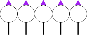
Exercise 2: Cottage
Here's the sample image. It is fine if your cottage in the woods does not exactly match ours.
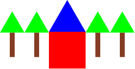
Exercise 3: The planets
Here's the sample image, which is an abstract representation of the planets of the solar system! Once again, it's fine if you don't match exactly. However, you should emulate the drop shadows behind each planet and try to approximate the relative size and colors of the planets.
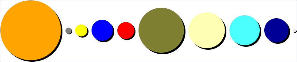
Exercise 4: Triangles
Yup, it's another image!
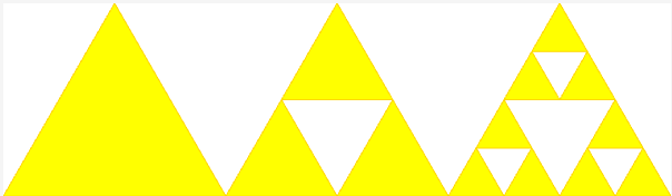
Writing your own procedures
In today's reading, we explore why and how to define your own procedures in Scheme.
Introduction
As you may recall from the introduction to algorithms, the ability to write subroutines is one of the key components of algorithm design. Subroutines typically have a name that we use to refer to the subroutine, zero or more parameters that provide the input to the subroutine, and a set of instructions (an expression in Scheme) for doing the computation. That is, a subroutine is just an algorithm that has been named and "parameterized".
For example, we might want to define a procedure, square, that takes as input a number and computes the square of that number.
(square 5)
(square 1.5)
(square 0.333)
(+ (square 0.5) (square 0.333))
(square (square 2))
As you may have noted, square can have multiple meanings. If
we're making drawings, it could also mean "make a square". Let's
consider an example.
(import image)

(square 50 "solid" "red")
(square 25 "solid" "blue")
(above (square 60 "solid" "red")
       (beside (square 40 "solid" "blue")
               (square 40 "solid" "purple")))
As you may recall, the image library already defines a square procedure, so it's unlikely to be a good idea for us to define our own square procedure, whether for numbers or images.
More generally, when we choose names in Scheme, we should try not to conflict with existing names.
Sometimes Scheme will stop us from reusing a name; other times it will blithely move along, letting us break things through such reuse.
So, how do we define these procedures? Read on and see.
Defining procedures with lambda
Scheme provides a variety of mechanisms for defining procedures.
We will start with the most general, which uses the keyword lambda, which means "procedure".
The lambda mechanism is relatively straightforward.
As you may recall, we typically think of a procedure as having three main aspects: The name we use to refer to the procedure, the names of the parameters (inputs) to the procedure, and the instructions the procedure executes.
Here is the general form of procedure definitions in Scheme, at least as we will use them in this class. Scheme does not require the indentation, but it makes it much easier to read and we will require it in this course.
(define <identifier>
  (lambda (<parameters>)
    <expression>))
You've already seen the define; we use define to name things.
In this case, we're naming a procedure, rather than a value.
The <identifier> part is straightforward; it's the name we will use to refer to the procedure.
The "lambda" is a special keyword in Scheme to indicate that "Hey! This is a procedure!".
Lambda has a special place in the history of mathematical logic and programming language design and has meant "function" or "procedure" since the early days of formal logic.
Lambda is special enough that the designers of Scamper chose it for the icon.)
The <parameters> are the names that we give to the inputs.
For example, we might use the names side-length and color for the inputs to our "make a square of s certain color" procedure. Similarly, we might use the name x for the input to the "square a number" procedure.
Finally, the <expr> is a Scheme expression that is the computation that the function performs when called.
Let's look at a simple example, that of squaring a number.
(define square-number
  (lambda (x)
    (* x x)))
Mentally, most Scheme programmers read this as something like
square-numbernames a procedure that takes one input,x, and computes its result by multiplyingxby itself.
Let's also look at some examples of using our new procedure.
(define square-number
    (lambda (x)
      (* x x)))
(square-number 5)
(square-number 0.5)
(square-number (square-number 2))
square-number
You may note in the last line that when we asked Scamper for the "value" of square-number, it told us that it's a function.
Compare that to other values we might define.
(import image)
(define x 5)
x
(define phrase "All mimsy were the borogoves")
phrase
(define red-square (rectangle 75 75 "solid" "red"))
red-square
(define multiply * )
multiply
In every case, Scamper is showing us the value associated with the name. In some cases, it's a number. In some cases, it's a string. In some cases, it's an image. And, in some cases, it's a procedure.
How does the procedure we've just defined work?
Here's one way to think about it: When you call a procedure you've defined with lambda, Scamper substitutes in the arguments in the procedure call for the corresponding parameters within the instructions.
After substituting, it evaluates the updated instructions.
For example, when you call (square-number 5), Scamper substitutes 5 for x in (* x x), giving (* 5 5).
It then evaluates the (* 5 5), computing 25.
What about a nested call, such as (square-number (square-number 2))?
As you may recall, Scheme evaluates nested expressions from the inside out.
So, it first computes (square-number 2).
Substituting 2 in for x, it arrives at (* 2 2).
The multiplication gives a value of 4. The (square-number 2) is then replaced by 4.
Scamper is then left to evaluate (square-number 4).
This time, it substitutes 4 in for the x, giving it (* 4 4).
It does the multiplication to arrive at a result of 16.
We might show the steps as follows, with the --> symbol representing
the conversion that happens at each step.
    (square-number (square-number 2))
--> (square-number (* 2 2))
--> (square-number 4)
--> (* 4 4)
--> 16
What about the colored squares?
If we want a procedure to make squares, we'll just call the rectangle procedure, using the same value for the width and height.
(import image)

(define color-square
  (lambda (side color)
    (rectangle side side "solid" color)))
What happens if we call color-square on inputs of 50 and "red"?
Scheme substitutes 50 for side and "red" for color, giving us (rectangle 50 50 "solid" "red").
And, as we saw in the examples above, that's a red square of side-length 50.
(import image)

(define color-square
  (lambda (side color)
    (rectangle side side "solid" color)))

(color-square 50 "red")
Another example
The square is a relatively simple example. Consider, for example, the following definition of a simple drawing of a house.
(import image)

(overlay/align "middle" "bottom"
             (overlay/align "left" "center"
                            (circle 3 "solid" "yellow")
                            (rectangle 15 25 "solid" "brown"))
             (above (triangle 50 "solid" "red")
                    (rectangle 40 50 "solid" "black")))
What if we want to make houses with different sizes or colors? We could copy and paste the code. However, if we changed our mind about how to structure our houses, we'd then have to update every copy. We'd be better off writing a procedure that takes the size and color as parameters.
How would we write house?
That's a question for another day.
Or perhaps for the lab.
For now, let's consider a simpler version, one that does not include the door. Remember: Decomposition is your friend! If we did not care about resizing the house, we might just write an expression like the following.
(import image)

(above (triangle 50 "solid" "red")
       (rectangle 40 50 "solid" "black"))
But we'd like to "parameterize" the code to take the size as an input.
Let's say that the size corresponds to the side-length of the triangle (or the height of the main body of the house).
We will replace each 50 by size and replace 40 by (* 4/5 size).
Let's see how that works.
(import image)

(define simple-house
  (lambda (size)
    (above (triangle size "solid" "red")
           (rectangle (* 0.80 size) size "solid" "black"))))
(simple-house 20)

(simple-house 30)
The next step might be to add parameters for the color of the body and the color of the roof.
Zero-parameter procedures
We've written procedures so that they take one or more parameters. However, there are also advantages to writing procedures that take no parameters. For now, just remember it's a possibility. In the future, you'll see what it's useful.
Some benefits of procedures
As you may have figured out by now, there are many benefits to defining your own procedures.
One of the most important is clarity or readability.
Another programmer will likely spend less effort understanding (simple-house 20) than they will trying to understand the more complex above expression involving triangles and rectangles.
The should be able to see that the first is intended to be a house.
The second could be anything, at least until you see it.
(As you may recall from the decomposition lab, the code to make a simple tree and the code to make a simple house look very similar.)
As importantly, the other programmer may also find it easier to write programs using simple-house than the much longer series of expressions.
By using a name for a set of code, we are employing the concept of abstraction.
That is, because the person calling the procedure knows what the procedure does rather than how it achieves that result, we have abstracted away some of the details.
Of course, for someone to know what the procedure does, you need to choose a good name.
img1 tells us very little, other than that it's an image.
house or tree gives us much more of a sense of what the procedure does.
Be thoughtful in your choice of procedure names.
(Also be thoughtful in your choice of parameter names---and any names, for that matter.)
There are benefits to abstraction and the use of procedures other than readability. For example, it may be that you discover a more efficient way to do a computation. If you've written the same code for the computation throughout your program, you'll have a lot of code to update. But if you've created a procedure, you need only update one place in your code, the place you've defined the procedure.
There are other ways in which procedures make us more efficient. For example, if we decide to change what our houses are like---say, by making the roof wider than the body of the house---we only have one place in our program to update.
As these examples suggest, using procedures to parameterize and name sections of code provides us with a variety of advantages. First, we can more easily reuse code in different places. Rather than copying, pasting, and changing, we can simply call the procedure with new parameters. Second, others can more easily read the code we have written, at least if we've chosen good names. Third, we can more easily update the procedures we've written, either to make them more efficient or to change behavior universally.
Using lambda without define
Scheme and related languages differentiate themselves from most other languages in that you can use lambda (or, more generally, subroutines) to define a procedure without bothering to name the procedure.
Recall, for example, that (lambda (x) (* x x)) represents "a procedure that takes one input, x, and computes x times x".
Since that's a procedure, Scheme permits us to write it in the "procedure slot" in an expression, as in
((lambda (x) (* x x)) 5)
What does that mean?
It means "take a procedure that takes one input, x, and computes x times x and apply it to 5, substituting the 5 for the x.
    ((lambda (x) (* x x)) 5)
--> ((lambda (x) (* x x)) 5)
--> (* 5 5)
--> 25
That doesn't seem very useful, does it?
And it's much harder to read, at least for now.
But it's worth it.
The power comes in when we use these "anonymous" procedures along with other tools.
For example, the map procedure which we covered briefly and will return to applies a procedure to each element of a list.
    (map (lambda (x) (* 3 x)) (list 1 2 3))
--> (list ((lambda (x) (* 3 x)) 1)
          ((lambda (x) (* 3 x)) 2)
          ((lambda (x) (* 3 x)) 3))
--> (list (* 3 1)
          (* 3 2)
          (* 3 3))
--> (list 3 6 9)
--> '(3 6 9)
Don't worry if you don't quite get this section! We'll return to the concepts in a week or two.
Self Checks
Check 1: A simple procedure
Write a procedure, (subtract2 val), that takes a number as input and
subtracts 2 from that number.
> (subtract2 5)
3
> (subtract2 3.25)
1.25
> (subtract2 "hello")
-:  Runtime error:
    A number? was expected, but a str was found
    In program: "hello"
Check 2: Building blocks (‡)
Write a procedure, (block color), that takes a color as input and builds a 40x20 "block" of the given color (a solid rectangle).
Check 3: Exploring steps
Show the steps involved in computing (square (subtract2 5)) and
(subtract2 (square 5)).
Q&A
These are questions gathered from previous reading responses.
Do we have to use they keyword lambda every time we want a procedure that takes in a parameter?
Yes. In fact, you have to use
lambdaif you want a procedure with no parameters.
What would be the difference between a zero parameter procedure and defined variable?
Right now, the biggest difference between a zero-parameter procedure and a defined variable are that you use them differently. The variable you use with its name; the procedure you put in parentheses.
Later in the semester, we'll see some differences. One difference is when the associated code is executed.
Acknowledgements
This section draws upon a reading entitled "Defining your own procedures" and an earlier reading entitled "Writing your own procedures" from Grinnell College's CSC 151.
It was updated in Spring 2022 to remove much of the discussion of zero-parameter procedures and to add a short section on anonymous procedures.
The house drawing was inspired by a more sophisticated house drawing from the Scheme Image Guide.
Practice with procedures
In this lab, we explore techniques for writing procedures in Scheme.
Syntax to remember
- Defining names:
(define <name> <expression>). - Function expressions:
(lambda (<parameters>) <expression>). - Defining functions:
(define <name> (lambda (<parameters>) <expression>))
The lab
As in the previous lab (and future labs), you will work with a randomly assigned partner using a starter file.
Remember to employ good pair programming practices as discussed in the previous lab!
- One person, the driver, is in control of keyboard. They focus on the immediate task of designing and coding a solution, speaking aloud about their design thoughts as they work.
- The other person, the navigator, acts as a reviewer. They observe and think more about strategic architectural issues. They look for potential issues and raise them with the driver. They are also responsible for keeping track of the time spent on the problem.
Work
All of the instructions are in the file. Switch to that now.
Acknowledgements
The checkerboard example comes from a very old version of CSC 151. We are no longer sure which member or members of the department wrote it.
Bits and parts of this lab come from procedure labs from other versions of CSC 151.
Assessment #2: working with the basic datatypes
In this mini-project, you will write a variety of procedures that explore various aspects of the basic datatypes you learned about this past week.
For this project, you will submit one file: basic-datatypes.scm.
Some background
As our programs get more complicated, the structure of our code and good names and formatting are not enough to make our code readable and correct. We need to rely on extrinsic means to ensure these things. To ensure that our code is readable, we use documentation to capture aspects of our code that are not obvious upon inspection. To ensure that our code is correct, we use tests that codify the correctness our programs through concrete examples.
During our week on software engineering fundamentals, we'll discuss these concepts in more detail. For now, we'll employ some basic documentation and testing for our program.
Documentation
For each function that you write in this mini project, include a function comment that captures the types of the function as well as describes its output in a sentence or two. For example, here is a function comment for a function that finds the minimum of three numbers:
;;; (min x y z) -> real?
;;;   x : number?
;;;   y : number?
;;;   z : number?
;;; Returns the minimum of x, y, and z
(define min-of-three
  (lambda (x y z)
    (cond
      [(and (<= x y) (<= x z))
       x]
      [(and (<= y x) (<= y z))
       y]
      [else
       z])))
The function comment is a stylized comment that consists of the following three components:
(min x y z) -> number?: the signature of the function which names its arguments and describes the output type of the function. In Racket, we express the types with the predicate functions that we use in code to test whether an expression has that type. For example, this signature says thatminhas three arguments,x,y, andzand that it produces a number (as tested by thenumber?function).x : number? ...: the types of each of the parameters mentioned in the signature. Like the return type of the function, we document the types of the parameters with the predicates that we would use in code to test values of those types.Returns the minimum of x, y, and z: finally, we include a brief sentence or two description of the behavior and output of the function. Here, the behavior of the function is simple, so we comparatively have little to say: the function returns the minimum of its arguments.
Tests
Up until this point, we have asked you to experiment with the functions that you write in the explorations window to check for correctness. This has the upside of being fast, but if you change your code, you need manually type in all those tests again which is tedious (which in turn makes it less likely you'll recheck the correctness of your code). A better solution is to codify your tests in your code so that you can rerun the tests at will.
During our unit on software engineering fundamentals, we'll introduce you to a library that makes test authoring and execution a breeze. For now, we'll simply have you call your functions on a variety of inputs within your file. For example, the reading on [characters and strings]({{ "/readings/strings.html" | relative_url }}) introduced a function that tests whether a value is a lowercase character:
(define lower-case-char?
  (lambda (x)
    (and (char? x)
         (char-lower-case? x))))
To test this function, we can call this function on several inputs and verify that the function behaves as expected. Note that we should choose a variety of inputs that exercise the different possibilities that the code considers, for example:
(lower-case-char? 5)    ; #f
(lower-case-char? #\a)  ; #t
(lower-case-char? #\C)  ; #f
(lower-case-char? "a")  ; #f
Setting up your file
You will have one file for this assignment, basic-datatypes.scm.
Here's the start of the file.
;; CSC-151-NN (TERM)
;; Mini-Project 2: Working with the basic datatypes
;; YOUR NAME HERE
;; YYYY-MM-DD
;; ACKNOWLEDGEMENTS:
;;   ....

(import image)
(import music)
Part 1: String Utilities
As you have likely discovered by now, the built-in Scheme procedures don't always immediately do what we want.
For example, although we can use a combination of integer? and string->number to determine if a string contains only digits, we would prefer not to write (integer? (string->number str)) again and again and again, particularly since we might later realize that that solution is not perfect.
When most programmers discover that they need to do the same thing again and again? They create a library of utility procedures that they plan to use in other procedures. Although you are just beginning your experience as a Racket programmer, you will still find it useful to create your own set of utilities.
For each of the following functions, do the following:
{:type="a"}
- Write several tests that describe how the function should work. Note that you haven't written the function yet! While this seems backwards, this test-driven design is useful in the design process to help you concretize the behavior of a function.
- Write documentation for the function as outlined above. Again, you haven't written the function yet! Documenting before you implement a function is another useful technique to solidify a design before you go to implementation.
- Finally, implement the function! In implementing your function, you will learn new things about the design, correct mistakes, etc., so you should update your tests and documentation accordingly.
In your tests, make sure to consider edge cases the exercise the "boundaries" of your code, e.g., the string is empty or the string contains an unexpected character.
(increment-wrap n bound)takes a non-negative integernas input and returnsn+1except ifn+1exceedsbound(also a non-negative integer), then it returns0instead.(slight-trim str)takes a stringstras input and returnsstrand removes a single leading space and a single trailing space on the ends ofstr, if they exist.(starts-with? s1 s2)takes two stringss1ands2as input and determines ifs1start withs2.(ends-with? s1 s2)takes two stringss1ands2as input and determines ifs1ends withs2.
Part 2: Ehrenstein Illusions
(Credit to Marty Stepp and Stuart Reges from the University of Washington for creating the original version of this assignment!)
An Ehrenstein Illusion is an optical illusion consisting of a collection of concentric circles and a diamond contained in a box. While we write the code to create a diamond, the circles will cause the sides of the diamond to look wavy!
For this part of the mini-project, you will ultimately write the following function:
(ehrenstein length n box-color circ-color outline-color): creates an image that contains a single Ehrenstein illusion with side lengthlength,ncircles, with the givenbox-colorandcirc-colorfor the box color and circle color, respectively.outline-colordetermines the color of the outline of the circles and the diamond.
With these functions, you should reproduce the following images as definitions in your program.
-
ehrenstein-1: a single Ehrenstein illusion of length200,5circles, a"red"box,"yellow"circles, and"black"outline.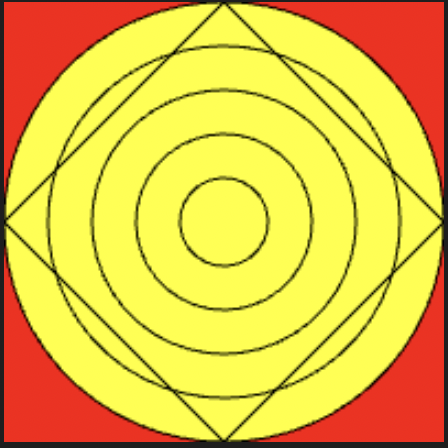
-
ehrenstein-2: a single Ehrenstein illusion of length100,10circles, an"aqua"box,"orange"circles, and"black"outline.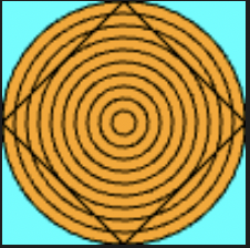
-
ehrenstien-3: a single Ehrenstein illusion of length50, no circles, a"white"box and circle, and"green"outline.
-
Critical to your decomposition of an Ehrenstein image is capturing the repetitive concentric circles. To do this, we'll incrementally develop a function
(ehrenstein-circles length n)that draws only the circle outlines of one Ehrenstein image. In doing so, we'll introduce how we can use the list datatype to perform repetitive computation. -
First let's step away from the code for a bit and develop a formula to compute the radius of an Ehrenstein circle given its position in the image. As a starting point, let's look at
ehrenstein-1which has5equally spaced concentric circles in a box of length200. Imagine assigning a number to each circle, an index, starting from0for the innermost circle and4for the outermost circle. Fill out the following table that lists each circle's index and that circle's corresponding radius.Circle Index Radius 0 ? 1 ? 2 ? 3 ? 4 ? To do this, recall that the circles are evenly spaced apart and the length of the entire image is
200. What must the distance be between each circle so that the circles are spaced evenly?From this table, derive a formula for the size of an Ehrenstein circle in terms of its index. To check your work, manually create the circles from
ehrenstein-1by using your computed radii combined with a call tooverlayto overlay each circle. To double-check your work, perform this exercise on the circles fromehrenstein-2(10 circles, length 100) and see if your formula works for this case, too.(Note: you do not need to include your table in your code anywhere! This is merely a design aid to help you in the successive parts of this homework! Additionally, make sure to comment out or remove your check code for your formula once you are confident it works.)
-
Next, let's put your formula to use. Write a function,
(circles-list length n)that creates a list of thenblack, outlined concentric circles that appear in an Ehrenstein image of the givenlength. To do so, you will need to put the following tools together:-
You first need to create a list containing the indices of the circles. To do so, the
(range n)function will be useful.(range n)produces a list of numbers in the range0ton-1. -
With a list of the indices in hand, you then need to transform each index into its corresponding Ehrenstein circle. To do so, you will need to use the
(map func lst)function which takes two arguments as input:- The first is a function
funcwhich takes an element of the list as input and transforms it in some way. - The second is the list
lstwhose elements will be transformed byfunc.
In other words,
maptakes a function that transforms a single element and uses it to transform an entire list of elements by applying the function to each element uniformally. - The first is a function
I recommend before trying to write
circles-listto try out examples ofrangeandmapon your own to get a sense of how they work. Importantly, keeping in mind that alambdaexpression is exactly that, an expression, we can callmapas follows to increment all the elements of a list:(map (lambda (n) (+ n 1)) (list 1 2 3 4 5))In this example, the provided
lambdatakes its argumentnand returnsn+ 1.mapwill apply this function to every elements of the list containing the numbers1through5. The result is the list(list 2 3 4 5 6).For our purposes, the
lambdawe provide tomapought to take an indexias input and produce a single Ehrenstein circle as output according to the formula you derived in the previous part. -
-
At this point, we have a way to generate a list of circles of the correct size. We must now combine them using one of the appropriate
imagefunctions that combines images together into a single image. However, these functions, e.g.,beside, expect the images to come in as individual arguments instead of a single argument that is a list. The function(apply func args)helps us use a list of values as the input to a function that takes multiple arguments. To useapply, we simply pass in thefuncthat takes multiple arguments and the list of argumentsargs. For example, the call(apply beside (list circ1 circ2 circ3))has the same effect as calling(beside circ1 circ2 circ3)for the images bound tocirc1throughcirc3. But now, we can callbesideand other functions like with it with alist!Use
applyalong withcircles-listto finally implement(ehrenstein-circles length n)! -
Finally, use
ehrenstein-circlesto complete the implementation ofehrensteinas described at the beginning of this part!
In addition to writing these functions, you should:
- Demonstrate that your
ehrensteinfunction works by calling the function at least three times at the end ofbasic-datatypes.scmwith various inputs. - Appropriately decompose your function into smaller functions as you identify different sub-components of the image.
- Give complete documentation strings for all functions that you write.
Submitting your work
Turn in your completed basic-datatypes.scm file to Gradescope.
Computation via Expressions
While it is tempting to start diving into hacking immediately, it is easy to "learn" a programming language by following our intuition, but then become lost when our intuition fails us. Instead, we should take some time to not only build cool stuff, but also understand:
- The structure of the code we are writing and
- How our programs execute.
This work in ultimately building a mental model of computation of how Scheme programs operate will pay dividends as we ramp up the complexity of our programs as well as begin transitioning to other languages at the end of the course.
Syntax and grammar
Consider the following two sequences of English words.
- The rain in Spain falls mainly on the plains
- In on the the falls plains rain mainly Spain
Which of these sequences do you understand? Why?
The sequences both contain the same words, just in different orders. However, we recognize the first sequence as a valid sentence in the English language, whereas the second sequence seems to be purely random. Because the first sequence is a sentence, we can figure out the meaning of the collection of words by the rules of sentence formation in English:
- Generally speaking, the subject of the sentence comes before the action that the subject performs. Thus, it is the "rain" that "falls" and not the other way around.
- We modify the subject and action with other fragments such as prepositional phrases ("in Spain") and adverbs ("mainly").
When words don't appear in the appropriate order, then it is at best, difficult, and at worst, impossible, to derive the intended meaning of the words.
The syntax of a language is its rules that govern whether a sequence of words is well-formed. You may have learned the syntax of English explicitly sometime during your prior education, or you may have picked it up experientially by observing others. Regardless, you adhere to the syntax of English so that others understand what you are saying.
The syntax of Scheme programs
While the second sequence of words above was in random order, you may have been able to understand the meaning of the words to some degree. This is because you are equipped with all sorts of cues and heuristics for infusing such sequences with meaning. Unfortunately, as we saw during our first day of class, computers are not natively equipped with such skills. Recall that:
Computers will do exactly what you tell them to do and nothing more!
Thus, we don't have the luxury of being lax in how we form programs. Our programs must adhere to the syntax of the programming language we are writing precisely!
This might be an impossible task in English because of the complexity and ambiguity of the language. Luckily, Scheme's syntax is much more compact and concise than English. So with some attention to detail, we can quickly learn how to form syntactically valid Scheme programs!
Expressions
The main syntactic form of Scheme programs is expressions.
Definition (Expression): an expression is a program fragment that evaluates to a value.
Definition (Value): a value is an expression that no longer takes steps of evaluation.
You have encountered expressions before when studying elementary math: arithmetic features numeric expressions that evaluate to numeric values. For example:
- \( 1 + 1 \) is a numeric expression that evaluates to the value \( 2 \).
- \( 3 \times (5 - 2 + 1) \) is a numeric expression that evaluates to the value \( 12 \).
- \( 32 \) is a numeric expression that is, itself, a value.
What is the syntax of an arithmetic expression? Well, numbers, themselves, are valid arithmetic expressions such as \( 32 \). And we can "join" together two numbers together with an operator, e.g., \( 1 + 1 \). But we're not constrained to numbers---we can take any pair of arithmetic expressions and join them with an operator to form a larger expression. For example, \( 1 + 1 \) and \( 3 - 2 \) are both valid expressions, so \( 1 + 1 - 3 - 2 \) is also valid! Note that parentheses here are used to be clear about how the different operators and operands associate, so we can also write \( (1 + 1) - (3 - 2) \) to be explicit.
In general, we can write down the rules of valid arithmetic expressions concisely. An arithmetic expression is either:
- A number or
- Two arithmetic expressions joined by an arithmetic operator in the middle (\( + \), \( - \), \( \times \), and \( \div \)).
As you saw in the last class's reading, Scheme's expression forms are different than traditional arithmetic. Rather than writing the operator between expressions in infix style, we write the operator for Scheme expressions in prefix style:
(+ 1 1)is a Scheme expression that computes the same value as \( 1 + 1 \).(* 3 (+ (- 5 2) 1))is a Scheme expression that computes the same value as \( 3 \times (5 - 2 + 1) \).32is a Scheme expression that computes the same value as \( 32 \).
Note that unlike arithmetic, we always surround our non-number expressions with parentheses. This is both a blessing and a curse. It is a blessing because this makes the order operations of a Scheme expression clear. It is a curse in that we have to write a lot of parentheses! We'll talk about how we can manage the complexity parentheses with appropriate style choices in our source code in later readings.
This infix versus prefix distinction is the primary difference between Scheme and arithmetic expressions. The rules or syntax of valid Scheme expressions are as concise as their arithmetic variants. An arithmetic Scheme expression is either:
- A number or
- An arithmetic operator followed by two Scheme expressions surrounded by parentheses.
It might be difficult to follow the language of the second bullet precisely, so it is useful to write out a sort of template that captures what the rule is conveying:
(<operator> <expr1> <expr2>)
Here, <operator> is a placeholder for any arithmetic operator and <expr1> and <expr2> are placeholders for any Scheme expression.
We call <expr1> and <expr2> sub-expressions of the overall expression.
Beyond arithmetic expressions
Of course, our last reading quickly moved from arithmetic to drawings, so we need our rules for Scheme expressions to generalize accordingly. Let's look at one of these expressions from our previous reading:
(circle 60 "outline" "blue")
What's different between this expression that produces a circle versus the arithmetic Scheme expression we studied earlier?
- The "operator" is no longer a symbol. Instead, it is a name or identifier.
- There are more than two operands to this
circleoperation. - The operands are no longer just numbers, they also include these words-in-quotes, strings.
We'll learn more about strings next week when we look at the primitive types of Scheme. For now, think of them as another sort of value we can perform computation over.
Given these observations, how can we generalize our rules for Scheme expressions accordingly? We'll make the following changes:
- We will not restrict ourselves to only arithmetic operations, we will allow any identifier as the operation to be performed! Not all identifiers will be valid operations when we go to execute our program, but in terms of forming a syntactically valid Scheme expression, we will allow any identfier as the operation.
- We will allow any number of arguments to our operations in a syntactically correct expression. Again, some operations will have restrictions on the number of arguments given to it that we will discover when we execute our program.
Our template for describing expressions that perform operations now looks like this:
(<identifier> <expr1> ... <exprk>)
Where the <expr1> ... <exprk> represents a sequence of sub-expressions separated by whitespace.
For example, in the example expression above:
circleis the identifier.60is the first sub-expression."outline"is the second sub-expression."blue"is the third sub-expression.
Putting everything together, we can write down the syntax of well-formed Scheme expressions as follows:
Definition (Well-formed expressions): a well-formed Scheme expression is either:
- A number,
- A string of the form
"<text>", or - An operation of the form
(<identifier> <expr1> ... <exprk>).
Note that this isn't it! We have much more to learn about Scheme, and we will revisit this definition and add and modify it as needed.
A mental model of computation for Scheme expression
It is one thing to form a syntactically valid English sentence. It is another thing to form a coherent, meaningful sentence! For example, the sentence:
I hefted the dishes below the hippo's qubits.
Is grammatically correct but non-sensible. For example, "hefting" (or lifting) dishes below something is odd. Furthermore, hippos don't have qubits to the best of our knowledge!
Alongside our knowledge of English syntax, we also have a sense of how to extract meaning out of grammatically correct sentences. Likewise, knowing the syntax of Scheme expressions is not enough. We must also know the "meaning" of expressions, i.e., how they compute.
Returning to arithmetic, we know from elementary mathematics how arithmetic expressions compute via repeated evaluation. For example, consider the expression \( 3 \times (5 - 2 + 1) \). According to the order of operations of arithmetic, we know that:
- \( 5 - 2 \) evaluates first to \( 3 \) because it is inside of parentheses and \( - \) and \( + \) have the same precedence, so we evaluate them in left-to-right order.
- Next, we evaluate \( 3 + 1 \) to \( 4 \).
- Finally, we evaluate \( 3 \times 4 \) to \( 12 \).
We can write this sequence of steps more concisely as follows:
\begin{align} &\; 3 \times (5 - 2 + 1) \\\ \longrightarrow &\; 3 \times (3 + 1) \\\ \longrightarrow &\; 3 \times 4 \\\ \longrightarrow &\; 12. \end{align}
Observe that our procedure for evaluating an arithmetic expression is:
- Find the next subexpression to evaluate according to the order of operation rules.
- Evaluate that subexpression to a value.
- Substitute the value for the subexpression that produced it in the overall expression.
These three steps taken together form a single step of evaluation. We repeatedly take steps of evaluation until the overall expression is a value. This model of arithmetic computation is also called a substitutive model of evaluation due to the last step where substitute value for subexpression.
Scheme expressions operate in the same way as arithmetic expressions. However, as mentioned above, Scheme's unique syntax makes evaluation easier: because everything is parenthesized, there is no ambiguity as to which subexpression evaluates next. We just find the innermost parenthesized expression and evaluate it! Let's see how the equivalent Scheme expression evaluates:
    (* 3 (+ (- 5 2) 1))
--> (* 3 (+ 3 1))
--> (* 3 4)
--> 12
Substitutive evaluation is our mental model of computation for Scheme expressions! In summary:
Definition (Substitute evaluation for Scheme expressions): Scheme expressions take repeated steps of evaluation until they evaluate to a final value. A step of evaluation consists of:
- Finding the next subexpression to evaluate. The next subexpression is the innermost parenthesized expression, evaluating arguments to operators left-to-right.
- Evaluating that subexpression to a value.
- Substituting the value for the subexpression that produced it in the overall expression.
Self-Checks
Check 1: Syntax (‡)
Consider the following expression that produces a drawing:
(above (rectangle 60 40 "solid" "red")
       (beside (rectangle 60 40 "solid" "blue")
               (rectangle 60 40 "solid" "black")))
Write down a list of:
- The sub-expressions of the overall expression.
- All the identifiers in the expression.
- All of the numbers in the expression.
- All of the strings in the expression.
Check 2: Semantics (‡)
Write down the step-by-step evaluation of the following Scheme expression.
Note that (expt x y) computes x raised to the y power, i.e., \( x^y \).
(expt (- (* 3 5)
         (/ 20 2))
      (- (+ 2 8)
         6))
Check your work in Scamper.
Mental models of Scheme programs
In the reading, we developed an initial mental model of computation for Scheme programs by examining how expressions compute.
In today's lab, we'll gain practice using that model to predict the behavior of simple Scheme programs.
We'll then enhance that model with the define construct that we have seen throughout our readings.
Logistics
You will do most labs on the computer. You will submit those labs on Gradescope. In most cases, we will ask you to upload a file or to copy a procedure you've written. It is fine if the code does not work perfectly (or at all). Just let us know that you're aware of the problems. Most of the time, you will only turn in a few of the exercises.
Other labs, such as this one, you will do some/most of your work on paper and submit the paper.
Whether electronic or paper, labs are due before the next class. You can use a token to submit a lab late, but it must be in before before the subsequent class.
While we would prefer that you finish the lab with your partner, if you decide to finish the lab separately, you may do so. Please make sure to cite your partner when submitting the lab.
In most labs, we will have distinguished driver/navigator roles where:
- The driver is the person "at the keyboard." In the context of a paper-based assignment, they should be the one writing down a final solution.
- The navigator is the person guiding the navigator and checking their work.
Each exercise will designate person A or person B to be the driver. Person A should be the person closest to the board.
Preparation
a. Introduce yourself to your partner.
b. Grab a piece of paper from the back of the room. If you don't have your own pen, feel free to grab a pen, too.
c. One partner should log in to the computer and start Scamper along with these instructions.
Exercises
Exercise 1: Tracing Scheme expressions (A drives, B navigates)
Consider the following Scheme expression.
(* (+ 1 2) (- (* 3 4) (* 2 (+ 1 1 1))))
a. Write down a step-by-step evaluation of this expression (we call this a trace or evaluation trace). If you're not sure what we're asking for, grab one of the course staff (professor or mentors).
b. Scamper's stepping tool allows you to trace the execution of a program using our mental model of computation. Try it out by entering the program into Scamper, running the stepping tool (the "path" button to the right of the "play" button used to run a program), and comparing your results to the stepper.
Exercise 2: From Math to Scheme (alternating drivers)
For this exercise, alternate drivers between each expression.
Consider the following arithmetic expressions.
- \( 3 * (4 - \frac{1}{7}) \). (Driver A)
- \( 1 + (-2 + (3 + (4 + -5))) \). (Driver B)
For each of these arithmetic expressions.
- Translate the expression into an equivalent Scheme expression.
- Give the step-by-step evaluation of that Scheme expression to a final value.
- Check your work with Scamper's stepping tool.
Exercise 3: Parts of Expressions
For this problem, alternate drivers between each expression.
In the reading, we introduced the syntax of expressions. It is easy to think of program constructs as fixed elements that must appear exactly as-presented in our programs. However, these program constructs are far more like highly-composable building blocks that, provided we understand how they connect, we can put together however we would like in order to express our computations.
In this problem, we'll take a look at identifying the various parts of expressions of significant complexity. For each of the following expressions, identify:
- The non-trivial sub-expressions of the overall expression.
- The identifiers of the overall expression.
- All of the numbers of the overall expression.
- All of the strings of the overall expression.
In addition to this information, try to "read" the expression and in a sentence, describe what you believe the expression evaluates to. Check your work in Scamper:
; (a) (Driver B)
(string-length
  (string-append "hello"
                 " "
                 "world!"))
; (b) (Driver A)
(+ 32 (* 8 60) (* (/ 1 2) 4 (expt 60 2)))
; (c) (Driver B)
(odd? (length (string-split "4,9,10,11,2,3" ",")))
Finally, with your partner, review your results for parts (a) and (c) and consider this statement:
When reading Scheme expressions, read them "inside-out" or "right-to-left."
Explain why this statement makes sense given what you know about how expressions evaluate and how they are syntactically formed.
Exercise 4: Making a Statement (Driver A)
In our first Scheme work, we learned that define is a construct that allowed us to introduce identifiers or named values into our programs. Each identifier/name is associated with ("bound to") a value. (Some people call these "variables"; since they don't vary, we will try to avoid that name.)
> (define x 10) ; binds the identifier/name x to the value 10
> (+ x 1)
11
Let's go through the process of trying to understanding how define in Scheme programs.
Along the way we'll update our mental model of computation to account for what we observe in our experimentation.
Note that this problem is a microcosm of the language-learning experience.
As you learn new constructs and techniques, you'll find that your current understanding of how program works does not account for these things, and you will evolve your learning.
Usually this evolution amounts to abstracting your understanding so that it applies to more scenarios than before!
At first glance the define construct above looks similar to the operator form or function call form of expressions we identified in the reading:
(<identifier> <expr1> ... <exprk>)
If this was the case, this implies that we can use define anywhere an expression is considered.
For example, perhaps we can get the same effect as the code above by inlining the define into the addition:
> (+ (define x 10) 1)
- Try this example out in Scheme. What is the output that you receive or what errors are produced if the code is invalid?
- Develop two other examples of trying to use
defineas an expression, similar to the give example case. (You should write these down on the piece of paper.) For inspiration, try replacing a value in an expression you've written already with(define x <value>). - Write down the output or errors that you get in each case.
- Answer the following question based on your experience: Is the
defineform an expression?
Exercise 5: The syntax of define (Driver B)
From the previous exercise, you should have concluded that define is not an expression!
We certainly do not seem to be able to put a define form anywhere an expression is expected.
Consequently, we must ask ourselves: what syntactic category is a define and how does it relate to expressions?
It turns out that define is an example of a syntactic category distinct from expressions; it is a statement!
A statement is a construct that produces an effect in our program.
We'll have more to say about "effects" in our programs later in the course.
For now, we'll say that the "effect" of a define statement is simple: it binds a value to an identifier.
In the example that started this problem, we bound 10 to the identifier x.
Consequently, whenever we mention x in our program, we really mean the value that is bound to that identifier, 10 in this case.
First let's address the syntax of a define.
So we far, we have seen that define takes the following form:
(define <??> <??>)
Where we haven't quite defined what goes in either <??> yet.
We assumed that a define statements binds an identifier, so it stands to reason that the first placeholder should be an identifier:
(define <identifier> <??>)
With your partner, try out define statements with different potential identifiers and different things in the last position.
You should try out various constructs that you've learned in the reading so far, in particular, the different forms of expressions.
From your experimentation, describe in a sentence what can appear in the final position of a define statement and complete the syntax rule with the syntactic category allowed in that position.
Exercise 6: Potential complexities (alternating Drivers)
Now let's think about how define statements execute.
In short, we execute statements in our program in sequential fashion.
However, subtleties may arise in this execution model that we should consider.
For each of the following programs:
- Write down how you expect the following programs evaluate, step-by-step.
- Test your answers in Scamper.
- In a sentence or two, describe how the program executes and why the program ultimately behaves in the way that it does.
Note that some of these programs produce errors; that is intentional!
; (i) (Driver A)
(define x 5)
(define y (* 5 8))
(define z (+ 1 1))

(+ x y z)
; (ii) (Driver B)
(define x 20)
(define y (* x 20))
(define z (* y y))

(+ x y z)
; (iii) (Driver A)
(define x 10)
(define y (+ x z))
(define z (* x 2))

(+ x y z)
; (iv) (Driver B)
(define x 10)
(define y (+ x 1))
(define x (* y 2))

(+ x y)
Exercise 7: Explaining define
In your own words, explain how our Scheme interpreter deals with a sequence of (interleaved expressions and define statements).
That is, what does the Scheme interpreter do if you write some define statements and some expressions and some more define statements and some more expressions and so on and so forth?
For example, consider what it does with the following.
(define x 10)   ; define statement
(+ x x)         ; expression
(define y 11)   ; define statement
(sqr y)         ; expression
(sqr x)         ; expression
(define z 12)   ; define statement
(define a 1)    ; define statement
(+ x y z)       ; expression
Submitting your work
Write your names at the top of the page.
Hand the page to one of the course staff.
Mental models of computation
So far, we have introduced a number of features of the Scheme programming language including top-level definitions, procedure declarations, and procedure applications. We have also focused nearly exclusively on how to author programs using these tools, appealing to your intuition about these constructs to explain how they work.
We've also recently learned about the substitutive model of evaluation. Basically, to evaluate an expression, we evaluate all of the arguments to the function and then apply the function. For convenience, we've been doing this left-to-right. The self-referential nature of the model also means that we end up evaluating expressions from inner to outer.
As you might expect, procedures complicate matters. Our intuition and the model might not be enough when we run into some special situations (some folks call these "corner cases") that we may run into when writing Scheme programs.
For example, consider the following procedure definitions:
(define f (lambda (x) (+ x 1)))

(define g (lambda (y) (+ y 1)))
Are these two procedures equivalent?
Textually, the procedures f and g are nearly identical, but the names of the parameters are different.
Does this difference matter?
Our intuition says no: parameter names don't seem to matter in this regard.
For example, if we try out these procedures in the Interactions pane:
> (f 5)
6
> (g 5)
6
> (f -1)
0
> (g -1)
0
There's too many integers to test in this manner, but after a few checks of this sort, we feel pretty confident in our intuition.
However, what happens if we have the following situation:
(define x 100)

(define f (lambda (x) (+ x 1)))
What will (f 10) produce?
Two possible answers are:
101if thedefineed version ofxis used in the computation off.11if the value of10that is passed to the procedure is used.
But maybe the code produces an error because there are two different x's, and the computer gets confused.
Or even more bizarre, but not out of the realm of possibility: maybe the defineed x is now 10 or 11!
Which of these is the correct answer? We can, of course, run this code to find out:
> (f 10)
11
> x
100
But why is this the case? What rules govern the execution of Scheme programs and how can they explain this behavior?
Before going too much further, let's try a similar pair of procedures.
(define eff (lambda (x) (+ x x)))

(define gee (lambda (y) (+ x y)))
Once again, we have a pair of procedures that seem to differ primarily in the name of the parameter.
Both add the parameter to x.
But is it the same x? What do you expect to happen for each of the following?
> (eff 10)

> (gee 10)
Before reading on, come up with a hypothesis.
Did you do so?
Great. Try it in your Scheme interpreter (DrRacket or Scamper or ...). You may also want to look at our notes at the end.
(Pause inserted in document so that you can check your answer by entering it in a Scheme interpreter, looking at the notes, or both.)
Since x does not always have a value, (gee 10) results in an error that x is undefined.
However, if x is defined, things will work fine.
The two functions will just be a bit inconsistent.
> (define x 100)
> (eff 10)
20
> (gee 10)
110
As you've likely concluded, understanding all that is going on is a bit complex.
In this reading, we'll consider a set of rules to help us better understand Scheme programs: a mental model of computation. This mental model will allow us to interpret many Scheme programs and accurately predict their results. Note that the mental model does not completely follow the implementation used in most Scheme interpreters; life is a bit too complex for that. However, it will help you understand most small programs. And we will extend the model throughout the semester.
Expressions
As we've seen, expressions lie at the core of Scheme. Expressions are syntactic constructs that evaluate to values. We are intimately familiar with expressions already: they form the basis of computation in arithmetic! For example, here is an arithmetic expression:
\[ 3 × (8 + 4 ÷ 2) \]
This expression evaluates to a final value, \( 30 \). We say that \( 30 \) is a value: it is an expression that no longer takes any steps of evaluation.
The analogous Scheme code is also an expression:
> (* 3 (+ 8 (/ 4 2)))
30
This extends to Scheme code that doesn't involve numbers at all!
(> (string-upcase (string-append "hello world" "!!!"))
"HELLO WORLD!!!"
Here the expression produces a string as output---the upper-case version of the string resulting from gluing "hello world" and "!!!" together.
A substitutive model of evaluation
The process of determining the value that an expression produces is called evaluation. The evaluation of expressions is the primary way that we perform computation in Scheme! But how do expressions evaluate? We determine how expressions evaluate by applying two basic sets rules:
- Rules of precedence that tell the order in which to evaluate operators.
- Associativity rules that tell us how the arguments to operators bind when chained together.
For arithmetic, we know that division and multiplication are evaluated before addition and subtraction. Furthermore, expressions in parentheses are evaluated first, irrespective of the operators involved. Finally, we typically expect that the arithmetic operators are left-associative resulting in a left-to-right evaluation order.
  3 × (8 + 4 ÷ 2)
= 3 × (8 +   2  )
= 3 ×     10
= 30
At every step of evaluation,
- We determine the sub-expression to evaluate next based off of our rules.
- We evaluate that sub-expression to a value.
- We substitute the resulting value for that sub-expression to create a new, slightly simplified expression.
We then repeat this process until we arrive at a final value.
While we may find Scheme's syntax arcane at first, it has one major benefit: There is only one rule for determining order-of-operations for expressions! That rule is straightforward: evaluate the arguments to a procedure before appling the procedure! (Some of us say "evaluate the innermost parenthesized expression first".) There is nothing else to know. Or almost nothing else to know. Let's see how that works for the Scheme version of this arithmetic expression:
    (* 3 (+ 8 (/ 4 2)))
--> (* 3 (+ 8    2  ))
--> (* 3      10     )
--> 30
(Note that we use the symbol --> to denote that one expression in Scheme evaluates or steps to another expression.)
Perhaps it would've been better in grade school if you were introduced to Scheme-style infix notation for arithmetic operations first. There are fewer rules to memorize, after all.
Okay, perhaps it's not quite that simple. What happens if a a procedure is called with multiple arguments, each of which is an expression?
(* (+ 1 2) (+ 4 1))
We need to evaluate the (+ 1 2) before we do the multiplication.
We need to evaluate the (+ 4 1) before we do the multiplication.
But which of those to should we do first?
Generally, it doesn't matter.
Let's check.
First, we'll evaluate the first argument first.
    (* (+ 1 2) (+ 4 1))
--> (* 3 (+ 4 1))
--> (* 3 5)
--> 15
Next, we'll evaluate the second argument first.
    (* (+ 1 2) (+ 4 1))
--> (* (+ 1 2) 5)
--> (* 3 5)
--> 15
You may not be surprised to discover that we got the same result in each case. But it turns out that we can't guarantee that in all programming languages. (We can't even guarantee it in Scheme, but we can guarantee it for most of the programs we write.) Nonetheless, for the time being, you can assume that the order in which we evaluate arguments does not matter, provided you evaluate arguments before you apply a procedure. And, even though the order does not matter, we will generally evaluate arguments left to right.
Definitions
We have a starting point.
We know how to evaluate expressions.
But expressions often involve identifiers (names).
In Scheme, we bind values to identifiers using define statements.
How should we mentally model define statements and the names they define?
One easy way to think about them is in terms of a table that tells us what value to use for each name.
When we see a define statement, we first evaluate the expression and then we put the name and the value in the table.
We tend to write that as name:value.
    ; Table: []
    (define x 5)
    ; Table: [x:5]
    (define y 17)
    ; Table: [x:5, y:17]
    (define z (* 2 3))
--> (define z 6)
    ; Table: [x:5, y:17, z:6]
What good is the table? The table informs how we evaluate expressions that consist only of variables (named values). When evaluating an expression, when the next expression to evaluate is a variable, we look in the table to find the value associated with the variables.
    ; Table: []
    (define x 10)
    ; Table: [x:10]
    (define y 2)
    ; Table: [x:10, y:2]
    (+ (* x 4) y))
    ; We need to evaluate the (* x 4) before we add
    ; We need to evaluate the x before we multiply.
    ; We look x up in the table
--> (+ (* 10 4) y)
    ; We need to evaluate the (* 10 x) before we add
--> (+ 40 y)
    ; We need to evaluate the y before we add
    ; We look y up in the table
--> (+ 40 2)
--> 42
Seems pretty straightforward. Right? What happens if we write an expression that involves a variable not in the table?
    ; Table: [x:10]
    (+ (* x 4) y))
--> (+ (* 10 4) y)
--> (+ 40 y)
    ; y is not in the table
    y: undefined
Note that these tables are mostly a notational convenience, designed to make it easier for us to figure out the value of expressions when we're tracing. However, most programming languages, including Scheme, also have a hidden form of table which basically does the same thing (that is, that associates values with variables names).
Procedures and the substitutive model
When we evaluate procedures, we have implicitly "carried out the behavior of the procedures" in our head and replaced the procedure call with the value. For example
    (+ 1 1)
--> 2
We know how addition works, so we can treat the evaluation of + as a single step.
Of course, if the arguments to + required evaluation first, we would need to carry that out according to our evaluation rules:
    (+ (+ 1 1) 8)
--> (+    2    8)
--> 10
The step-by-step evaluation of an expression to a final value is called the execution trace or just trace of a particular expression.
However, what happens when our procedures are those we have defined ourselves?
For example, something simple like double:
(define double
  (lambda (n)
    (* 2 n)))
How does an expression like (double (/ 6 3)) evaluate?
As a first order of business, we should evaluate its argument to a value.
    (double (/ 10 2))
--> (double 5)
Good!
Now how does (double 5) evaluate?
We proceed as follows:
- We substitute the body of the procedure for the procedure call in question.
The body of
doubleis(* 2 n)so we would replace(double 5)with(* 2 n). - Note that, on its own, the parameter
nis not defined! To patch this up, we also substitute each argument for its associated parameter in the body of the procedure. We pass5fornso we ultimately replace(double 5)with(* 2 5).
All of this occurs in one step of evaluation and afterwards, we continue evaluation of the expression as normal. So the complete evaluation of our original expression is:
    (double (/ 10 2))
--> (double    5)
--> (* 2 5)
--> 10
While this rule is simple, it covers almost all occurrences of procedures we'll see in Scheme! This is the beauty of a programming language at its core: a small set of rules governs a near, unimaginable set of behavior we can author in a computer program!
Definitions, tables, and procedures
We've separately considered models for the definitions that let us evaluate variables for procedures.
Let's also consider them together.
We know that (define var exp) evaluates the expression and the pairs it with the variable in a table.
So what happens when we write (define var (lambda (params) body))?
It turns out that Scheme does something a bit special with lambda expressions (expressions that begin with lambda). Instead of evaluating them further, Scheme stops evaluating until you need to apply the lambda expression. Then, and only then, does it do what we described above: We substitute it in for the name and then replace its named parameters (the "formals", in CS parlance) with the values of the corresponding arguments (the "actuals", in CS parlance).
It turns out that these model of operation means we can use lambdas without defining them. We'll leave that issue for a bit later in your education.
Self-checks
Check 1: Code tracing (‡)
Assume the existence of the following Scheme definitions:
(define add-3
  (lambda (x y z)
    (+ (+ x y) z)))

(define triple
  (lambda (n)
    (add-3 n n n)))
With these definitions, give the step-by-step evaluation (i.e., evaluation traces) for each of the following expressions. Please do this by hand; don't rely on the tools that might be part of your Scheme interpreter. Make sure to write down all steps of evaluation as required by our substitutive model of computation!
(+ 3 (* 5 (/ 2 (- 10 5))))(add-3 (* 2 3) (+ 8 3) (/ 1 2))(triple (+ 5 0.25))
Make sure to check your work by entering these expressions into your Scheme interpreter!
Appendices
Appendix A: eff and gee
What should we get for (eff 10)? Presumably, x gets the value 10, we add the two 10 values together, and end up with 20.
Let's check.
> (eff 10)
20
But what happens when we try (gee 10)? In that case, y gets the value 10. What value does x have? Unless we've defined x with define, it has no value. Perhaps we'll get an error.
> (gee 10)
. . x: undefined;
 cannot reference an identifier before its definition
Expressions and types
From our discussion of mental models of computation, we know that Scheme programs are composed primarily of expressions, program fragments that evaluate to values. What are the different kinds of values that expressions can evaluate to? In other words, what kinds of data can our Scheme programs manipulate? We've seen some examples already, e.g.,
-
Numbers:
(* 3 (- 1 5) (+ 2 4))
-
Strings:
(string-append "hello" "world!")
-
Images:
(import image)

(beside (circle 50 "solid" "blue") (square 25 "solid" "red"))
But are there others? What are the different categories of data we might operate over and how are they organized? In this reading, we focus on the different kinds of primitive values that we can manipulate in our Scheme programs.
Primitive vs. compound data
In computer programming, we can categorize the wide-range of data into two sorts:
- Compound data: data that is made up of other, smaller pieces of data.
- Primitive data: "indivisible" data, i.e., data that cannot be broken up into smaller pieces.
For example, consider representing a student in a computer program. A student has many potential pieces of data associated with them, e.g.,
- Name,
- Email,
- Student ID,
- Age,
- Hometown,
- Current GPA, and
- Current classes for the fall.
In this sense, students are examples of compound data. An individual student, from the perspective of a computer program, is made up of these parts.
In contrast, consider just the student's age. The student's age compromises of a single number, usually just a natural number, zero or a positive integer (non-fractional) quantity. At the level of abstraction we're working at, we think of numbers as indivisible units---unlike a student, a number isn't made up of small data. In this sense, numbers are examples of primitive data. Another term for primitive data are atomic data because they cannot be broken up any further.
Types
We intuitively recognize that these values:
3
0
-1
47
Are different from these values:
"hello!"
"csc151"
"world"
"47"
The primitive versus compound distinction allows us to categorize groups of data based on their "atomicity."
However, within these buckets are different categories of data.
We call such a category a type.
For example, the first set of values are all numbers whereas the second set of values are all strings.
We say that each of the values are instances of these types, e.g., 3 is an instance of the number type or 3 has type number.
Types of expressions
We assign types to particular values, e.g., 5 has type "number" (or, more
precisely, "exact integer").
Recall that a value is an expression that takes no further steps of evaluation.
We can define the type of any expression, not just values, as follows:
The type of an expression is the type of the value that the expression evaluate to.
Types of functions
For example (+ 1 1) is a non-value expression that has type number.
We know this because (+ 1 1) --> 2 and 2 is a number.
When we perform operations over data, e.g., addition through the + function, we must provide values of the appropriate type.
Here, + expects to be given at least one argument, all of which must be numbers:
(+ 1 3 5 7 9)
When a function is provided values of an appropriate type, a type error occurs when trying to run that function on those values. For example:
(+ 1 "hello")
Scheme realizes these type errors as contract violations when trying to execute the function.
Intuitively, we can think of + as specifying the following contract:
If you provide me with values that are all numbers, I will give you back a number that is the sum of those input numbers.
From this contract, we say that the type of the function is the expected type of its inputs and output.
For + the expected types of the inputs as numbers and the expected type of the output is a number.
For function types, the types of the inputs and outputs don't have to be the same, e.g.,
(string-length "hello world")evaluates to11. The type of the input tostring-lengthis a string and the output is a number (exact integer).(substring "hello world" 2 5)evaluates to"llo"---substringreturns the portion of the string starting with the character at the index (inclusive) denoted by the first argument and ends with the character at the index (exclusive) denoted by the last argument.substringtakes a string and two numbers as input and produces a string as output. (Note: the indices of a string start at 0, solis indeed the character at index 2!)
As you have likely noticed, keeping the type of a function in mind is really important for debugging your code.
For example, consider the following erroneous call to circle:
(import image)

(circle "red" "solid" 500)
If we recall that the type of circle is:
circleis a function that takes a number (the radius), a string or symbol (the fill), and string or symbol (the color) as input and produces an image as output.
We'll note that the problem with the code is that we've incorrectly interchanged the radius and the color!
Type mismatches of this sort are a common error in programming, especially when you start out. Whenever you write code, try to keep in mind:
What is the intended type of the expression that I am trying to write?
This mentality will bring you one step closer towards truly writing code in an intentional, purposeful fashion and not simply throwing random stuff at the wall and seeing if it works!
Primitive data in Scheme
The remainder of today's readings are broken up into readings for two of the major primitive types we see in Scheme:
- [Numbers]({{ "/readings/numbers.html" | relative_url }})
- [Characters and Strings]({{ "/readings/strings.html" | relative_url }})
For each of these primitives, we introduce the following concepts:
- What does a datum of this type represent?
- How do we make values of this type?
- What library functions are available for manipulating values of these types?
You do not have to memorize all of this information in one go as it is a lot of stuff! Instead, you should look initially to get the big picture: what broad sorts of operations are possible with each type of data and what can I expect to do? From there, you can always refer back to these readings and Scamper reference found in VSCode to find particular functions to achieve the effect you are looking for.
Self-checks
The readings on primitive data have a number of self-checks. Please complete the following self-checks for your reading question set for this collection:
- (‡) Numbers: Check 1 (Exploring exponentiation)
- (‡) Collating Sequences: Check 2 (Collating sequences)
Numeric values
In this reading, we examine a variety of issues pertaining to numeric values in Scheme, including the types of numbers that Scheme supports and some common numeric functions.
Introduction
Computer scientists write algorithms for a variety of problems. Some types of computation, such as representation of knowledge, use symbols and lists. Others, such as the construction of Web pages, may involve the manipulation of strings (sequences of alphabetic characters). Even when working with text, a significant amount of computation involves numbers. And, even though numbers seem simple, it turns out that there are some subtleties to the representation of numbers in Scheme.
As you may recall from our first discussion of data types, when learning about data types, you should consider the name of teach type, its purpose, how Scamper displays values in the type, how you express those values, and what operations are available for those values.
While it seems like "numbers" is an obvious name for this type, Scheme provides multiple kinds of numeric values. In each case, the purpose is the same: to support computation that involves numbers.
Categories of numeric values
As you probably learned in secondary school, there are a variety of categories of numeric values. The most common categories are integers, (numbers with no fractional component), rational numbers (numbers that can be expressed as the ratio of two integers), and real numbers (numbers that can be plotted on a number line). You also learned about complex numbers (numbers that can include an imaginary component) that arose when you solved polynomials with real coefficients.
In traditional mathematics, each category is a subset of the next category. That is, every integer is a rational number because it can be expressed with a denominator of zero, every rational number is a real number because it can be plotted on the number line, and every real number is complex because it can be expressed with an imaginary component of zero.
In contrast, Scamper does not readily distinguish the rational and real numbers. Instead, like most conventional programming languages, Scamper distinguishes between two broad classes of numbers:
- Integral values, i.e., numbers without a fractional component, e.g.,
427198. - Floating-point values, i.e., numbers with a fractional component, e.g.,
3.4170.
Importantly, because these numbers must be physically stored in a computer somewhere, they are necessary bounded values, i.e., there are limits to the sizes of values these numbers can represent.
Recall that some numbers, e.g., the irrational numbers such as \( \pi \), have infinite decimal expansions. A consequence of the bounded nature of numbers in a computer program is that we have to represent numbers like \( \pi \) as approximations. In other cases, when we perform some computations involving infinite fractional components, we may induce round-off error because we have to store these infinite values using a finite amount of space.
When Scamper displays a number that is a floating point value, it includes a decimal point, an exponential component in the result, or both.
(sqrt 2)
(expt 3.0 100)
Why is the square root of 2 approximated? Because it's impossible to represent precisely as a finite decimal number. That means that Scamper approximates it. And, because it's approximated, our calculations using that result will also be approximate.
(* (sqrt 2) (sqrt 2))
The decimal sign warns us that we are straying into the realm of estimations and approximations.
In contrast, integer computations are always exact provided that we don't produce numbers that are bigger than the maximum size of an integer in Scamper. In those cases, Scamper will automatically move to a floating-point representation which is approximate.
(+ 1 1)
(/ 10 2)
(* 426198421879421897412 4782147894721489712)
You can express values to Scamper using similar notation. That is, when you want a precise integer value, you do not include a decimal point or the exponent. When you want a floating-point number, you include the dot and/or exponent.
-3
0.5
(+ 1 1e-7)
In general, programmers tend to model objects in the world using integers because they provide precise, predictable results. When we use floating-point numbers, we have to be highly aware of their approximate nature and go out of our way to ensure our programs are correct in spite of those limitations. In fact, whole areas of mathematics, e.g., applied computational mathematics, are dedicated to studying algorithms that perform tasks with floating-point numbers that minimize errors!
When describing the procedures that work with numbers, we should try to
describe how the type of the result depends on the type of the input. For
example, the addition operator, ,+ provides an integer result only when all
of its inputs are integers. Note that Scamper will gladly give an integral
result if it can deduce that one of the arguments is actually integral, even
when written as a floating-point number.
(+ 2 3 4)
(+ 2 3.0 4)
(+ 2 1e-3 5)
(+ 2 3.0 -3.1)
Numeric operations
You've already encountered the four basic arithmetic operations of
addition (+), subtraction (-), multiplication (*), and
division (/). But those are not the only basic arithmetic
operations available. Scheme also provides a host of other numeric
operations. We'll introduce most as they become necessary. For now,
we'll start with a few basics.
Integer division
In addition to "real division", Scheme also provides two procedures that
handle "integer division", quotient and remainder. Integer division
is is likely the kind of division you first learned; when you divide one
integer by a number, you get an integer result (the quotient) with,
potentially, some left over (the remainder). For example, if you have
to divide eleven jelly beans among four people, each person will get two
(the quotient) and you'll have three left over (the remainder).
(quotient 11 4)
(remainder 11 4)
(quotient 15 5)
(remainder 15 5)
We also get sensible results when mixing floating-point and integer values.
(quotient 5.5 2)
(remainder 5.5 4)
Roots and exponents
As you've seen, Scheme provides ways to compute the square root of a number,
using (sqrt x) and to compute "x to the n" using (expt x n). When given
integer inputs, both return inexact results. Both will provide floating-point
results if the output demands it or if the inputs are floating-point numbers.
(sqrt 4)
(sqrt 4.0)
(sqrt 2)
(expt 2 5)
(expt 0.3 0.8)
What happens when we take the square root of a negative number? Recall that the result is a complex number, a number with the imaginary number .
(sqrt -2)
In Scamper, we get NaN which is a special number called Not a Number.
NaNs are produced by our math operations when they would end up producing
a non-real number.
Finding small and large values
Scheme provides the (max val1 val2 ...) and
(min val1 val2 ...) procedures to find the largest or smallest
in a set of values. Both of these procedures will produce an exact
number only when all of the arguments are exact. As you might expect,
the value produced will be an integer only when it meets the criterion
of being largest or smallest.
(max 1 2 3)
(max 3 1 2)
(max 2 1 3)
(max 1 2 3 1.5)
(min 3 1 2 4 8 7 -1)
Rounding
Scheme provides four different ways to round real numbers to nearby
integers. (round num) rounds to the nearest integer.
(floor num) rounds down. (ceiling num) rounds up.
(truncate num) throws away the fractional part, effectively rounding
toward zero.
(round 3.2)
(round 3.8)
(floor 3.8)
(ceiling 3.8)
(truncate 3.8)
(floor -3.8)
(truncate -3.8)
Self Checks
Check 1: Exploring exponentiation (‡)
In the examples above, we gave a wide variety of examples of the expt
procedure in action. Try expt on additional examples of your own design, and
try to cover all the possible combinations of integer, negative/non-negative,
and floating-point values to the function.
After you have done this, try to summarize as concisely as possible the
situations in which expt will produce:
- An integral result and
- A floating-point result.
Characters and strings
Computer scientists refer to text in many ways. A text file is a document stored on the file system in a computer that contains text. A string is a piece of text available within a computer program. And a character is the basic building block that we use to create strings. In this reading, we explore the representation of characters and strings in Scheme. In a subsequent reading, we will consider files.
As you may recall, there are five issues we typically consider as we encounter a new type: The name of the type, the purpose of the type, the way you express elements of the type, the way Scamper displays elements of the type, and the operations of the type. In this reading, we consider characters and strings, two of the important primitive data types in many languages. Characters are the building blocks of strings. Strings, conversely, are combinations of characters. Both characters and strings are useful for input and output.
About characters
A character is a small, repeatable unit within some system of writing -- a letter or a punctuation mark, if the system is alphabetic, or an ideogram in a writing system like Han (Chinese). Characters are usually put together in sequences that computer scientists call strings.
Although early computer programs focused primarily on numeric processing, as computation advanced, it grew to incorporate a variety of algorithms that incorporated characters and strings. Some of the more interesting algorithms we will consider involve these data types. Hence, we must learn how to use this building blocks.
Characters in Scheme
We've covered the name of this type (character) and its purpose (to represent the individual components of a string or other piece of text). What's next? How to represent characters.
As you might expect, Scheme needs a way to distinguish between many different but similar things, including: characters (the units of writing), strings (formed by combining characters), symbols (which look like strings, but are treated as atomic and also cannot be combined or separated), and identifiers (names of values). Similarly, Schemes needs to distinguish between numbers (which you can compute with) and digit characters (which you can put in strings).
In Scheme, a name for any of the text characters can be formed by writing #\
before that character. For instance, the expression #\a denotes
the lower-case a. Of course, lower-case a should be distinguished from
the upper-case A character, (denoted by #\A), from the symbol that you
obtain with 'a, from the string "a", and from the name a. Similarly,
the expression #\3 denotes the character 3 (to be distinguished from
the number 3) and the expression #\? denotes the question mark (to be
distinguished from a symbol and a name that look quite similar).
In addition, some characters are named by pound, backslash, and a longer
name. In particular, the expression #\space denotes the space
character, and #\newline denotes the newline character (the one that is
used to terminate lines of text files stored on Unix and Linux systems).
Collating sequences
In any implementation of Scheme, it is assumed that the available
characters can be arranged in sequential order (the "collating
sequence" for the character set), and that each character is
associated with an integer that specifies its position in that
sequence. In ASCII, the American Standard Code of Information
Interchange, the numbers that are associated with characters run
from 0 to 127; in Unicode, a more extensive character set intended
to support most languages, they lie within the range from 0 to
65535. (Fortunately, Unicode includes all of the ASCII characters
and associates with each one the same collating-sequence number
that ASCII uses.) Applying the built-in char->integer procedure
to a character gives you the collating-sequence number for that
character; applying the converse procedure, integer->char, to an
integer in the appropriate range gives you the character that has
that collating-sequence number.
The importance of the collating-sequence numbers is that they extend
the notion of alphabetical order to all the characters. Scheme provides
five built-in predicates for comparing characters (char<?, char<=?,
char=?, char>=?, and char>?). They all work by determining which
of the two characters comes first in the collating sequence (that is,
which one has the lower collating-sequence number).
The Scheme specification requires that if you compare two capital
letters to each other or two lower-case letters to each other, you'll
get standard alphabetical order: (char<? #\A #\Z) must be true, for
instance. If you compare a capital letter with a lower-case letter,
though, the result depends on the design of the character set. In ASCII,
every capital letter (even #\Z) precedes every lower-case letter (even
#\a). Similarly, if you compare two digit characters, the specification
guarantees that the results will be consistent with numerical order:
#\0 precedes #\1, which precedes #\2, and so on. But if you compare
a digit with a letter, or anything with a punctuation mark, the results
depend on the character set.
Handling case
Because there are many applications in which it is helpful to ignore
the distinction between a capital letter and its lower-case equivalent
in comparisons, Scheme also provides case-insensitive versions of
the comparison procedures: char-ci<?, char-ci<=?, char-ci=?,
char-ci>=?, and char-ci>?. These procedures essentially convert all
letters to the same case before comparing them.
There are also two procedures for converting case, char-upcase and
char-downcase. If its argument is a lower-case letter, char-upcase
returns the corresponding capital letter; otherwise, it returns the
argument unchanged. If its argument is a capital letter, char-downcase
returns the corresponding lower-case letter; otherwise, it returns the
argument unchanged.
More character predicates
Scheme provides several one-argument predicates that apply to characters: (We'll explain more about predicates in a subsequent reading.)
char-alphabetic?determines whether its argument is a letter (#\athrough#\zor#\Athrough#\Z, in English).char-numeric?determines whether its argument is a digit character (#\0through#\9in our standard base-ten numbering system).char-whitespace?determines whether its argument is a "whitespace character", one that is conventionally stored in a text file primarily to position text legibly. In ASCII, the whitespace characters are the space character and four specific control characters: tab, line feed, form feed, and carriage return. On most systems,#\newlineis a whitespace character. On our Linux systems,#\newlineis the same as line feed and counts as a whitespace character.char-upper-case?determines whether its argument is a capital letter.char-lower-case?determines whether its argument is a lower-case letter.
It may seem that it's easy to implement some of these operations. For
example, you might want to implement char-alphabetic? using a strategy
something like the following.
A character is alphabetic if it is between
#\athrough#\zor between#\Athrough#\Z
However, that implementation is not necessarily correct for all versions of Scheme: Since the Scheme specification does not guarantee that the letters are collated without gaps, it's possible that this algorithm treats some non-letters as letters. The alternative, comparing to each valid letter in turn, seems inefficient. It is also biased toward American English, making it inappropriate for languages with different alphabets. By making this procedure built-in, the designers of Scheme have encouraged programmers to rely on a correct (and, presumably, efficient) implementation.
(char<=? #\a #\n #\z)
(char-lower-case? #\n)
(char<=? #\a #\N #\z)
(char-lower-case? #\N)
(char<=? #\a #\ñ #\z)
(char-lower-case? #\ñ)
Note that all of these predicates assume that their parameter is a character. Hence, if you don't know the type of a parameter, you will need to first ensure that it is a character. For example,
(char-lower-case? #\a)
(char-lower-case? #\5)
(char-lower-case? 23)
(and (char? 23) (char-lower-case? 23))
(define lower-case-char? (lambda (x) (and (char? x) (char-lower-case? x))))
(lower-case-char? 23)
(lower-case-char? #\a)
String basics
We've now covered the five primary issues for the character type: Its name, purpose, representation and display (with pound and backslash), and some important operations. It is now time to turn our attention to strings, the longer pieces of text we can build with characters.
Once again, we've covered the name and the purpose quickly. Strings provide a mechanism for representing text by joining together a sequence of characters. (We even allow that sequence to have no characters; in that case, we call it the empty string.)
How do we express strings? Most strings can be expressed by
enclosing the characters they contain between plain double quotation
marks, to produce a string literal. For instance, "periwinkle"
is the nine-character string consisting of the characters #\p,
#\e, #\r, #\i, #\w, #\i, #\n, #\k, #\l, and #\e,
in that order. Similarly, "" is the zero-character string (the
null string or the empty string).
String literals may contain spaces and newline characters; when such
characters are between double quotation marks, they are treated like any
other characters in the string. There is a slight problem when one wants
to put a double quotation mark into a string literal: To indicate that
the double quotation mark is part of the string (rather than marking the
end of the string), one must place a backslash character immediately
in front of it. For instance, "Say \"hi\"" is the eight-character
string consisting of the characters #\S, #\a, #\y, #\space,
#\", #\h, #\i, and #\", in that order. The backslash before
a double quotation mark in a string literal is an escape character,
present only to indicate that the character immediately following it is
part of the string.
This use of the backslash character causes yet another slight problem:
What if one wants to put a backslash into a string? The solution is
similar: Place another backslash character immediately in front of
it. For instance, "a\\b" is the three-character string consisting
of the characters #\a, #\\ , and #\b, in that order. The first
backslash in the string literal is an escape, and the second is the
character that it protects, the one that is part of the string.
String operations
Scheme provides several basic procedures for working with strings:
The (string? val){:.signature} predicate determines whether its argument
is or is not a string.
The (make-string count char){:.signature} procedure constructs and
returns a string that consists of count repetitions of a single
character. Its first argument indicates how long the string should be, and
the second argument specifies which character it should be made of. For
instance, the following code constructs and returns the string "aaaaa".
(make-string 5 #\a)
The (string ch_1 ... ch_n){:.signature} procedure takes any number
of characters as arguments and constructs and returns a string
consisting of exactly those characters. For instance, (string #\H #\i #\!)
constructs and returns the string "Hi!". This procedure
can be useful for building strings with quotation marks. For example,
(string #\" #\") produces "\"\"". (Isn't that ugly?)
The (string->list str){:.signature} procedure converts a string
into a list of characters. The (list->string char-list){:.signature}
procedure converts a list of characters into a string. It is invalid
to call list->string on a non-list or on a list that contains values
other than characters.
(string->list "Hello")
(list->string (list #\a #\b #\c))
(Note: it looks like there is a bug with the interpreter used in
the reading. Individual characters are printed as $\h instead of #\h,
i.e., with a dollar sign instead of a hash!)
The (string-length str){:.signature} procedure takes any string
as argument and returns the number of characters in that string. For
instance, the value of (string-length "magenta") is 7 and the value of
(string-length "a\\b") is 3.
The (string-ref str pos){:.signature} procedure is used to select
the character at a specified position within a string. Like list-ref,
string-ref presupposes zero-based indexing; the position is specified
by the number of characters that precede it in the string. (So the initial
character in the string is at position 0, the next at position 1, and so
on.) For instance, the value of (string-ref "ellipse" 4) is #\p --
the character that follows four other characters and so is at position
4 in zero-based indexing.
Strings can be compared for "lexicographic order", the extension of
alphabetical order that is derived from the collating sequence of the
local character set. Once more, Scheme provides both case-sensitive and
case-insensitive versions of these predicates: string<?, string<=?,
string=?, string>=?, and string>? are the case-sensitive versions,
and string-ci<?, string-ci<=?, string-ci=?, string-ci>=?, and
string-ci>? the case-insensitive ones.
The (substring str start end){:.signature} procedure takes three
arguments. The first is a string and the second and third are non-negative
integers not exceeding the length of that string. The substring
procedure returns the part of its first argument that starts after the
number of characters specified by the second argument and ends after
the number of characters specified by the third argument. For instance:
(substring "hypocycloid" 3 8) returns the substring "ocycl" --
the substring that starts after the initial "hyp" and ends after the
eighth character, the l. (If you think of the characters in a string
as being numbered starting at 0, substring takes the characters from
start to end - 1.)
The (string-append str1 str2 ... strn){:.signature} procedure
takes any number of strings as arguments and returns a string formed by
concatenating those arguments.
(string-append "al" "fal" "fa")
The (number->string num){:.signature} procedure takes any Scheme number
as its argument and returns a string that denotes the number.
(number->string 23)
(number->string 1.2)
(number->string pi)
The (string->number str){:.signature} procedure provides the inverse
operation. Given a string that represents a number, it returns the
corresponding number. On some implementations of Scheme, when you give
string->number an inappropriate input, it returns the value #f
(which represents "no" or "false"). You are then responsible
for checking the result.
(string->number "23")
(string->number "1.2")
(string->number "0.000000000000000000000000001")
(string->number "")
(string->number "two")
(string->number "3 + 4i")
(string->number "3+4i")
The string-upcase and string-downcase procedures convert all of
the letters in the string to uppercase or lowercase..
(string-upcase "aLpHaBeTiCAL")
(string-downcase "aLpHaBeTiCAL")
Appendix: Representing characters
When a character is stored in a computer, it must be represented
as a sequence of bits ("binary digits", that is, zeroes and
ones). However, the choice of a particular bit sequence to represent
a particular character is more or less arbitrary. In the early days of
computing, each equipment manufacturer developed one or more "character
codes" of its own, so that, for example, the capital letter A was
represented by the sequence 110001 on an IBM 1401 computer, by 000001
on a Control Data 6600, by 11000001 on an IBM 360, and so on. This
made it troublesome to transfer character data from one computer to
another, since it was necessary to convert each character from the source
machine's encoding to the target machine's encoding. The difficulty was
compounded by the fact that different manufacturers supported different
characters; all provided the twenty-six capital letters used in writing
English and the ten digits used in writing Arabic numerals, but there
was much variation in the selection of mathematical symbols, punctuation
marks, etc.
ASCII
In 1963, a number of manufacturers agreed to use the American Standard Code for Information Interchange (ASCII), which is currently the most common and widely used character code. It includes representations for ninety-four characters selected from American and Western European text, commercial, and technical scripts: the twenty-six English letters in both upper and lower case, the ten digits, and a miscellaneous selection of punctuation marks, mathematical symbols, commercial symbols, and diacritical marks. (These ninety-four characters are the ones that can be generated by using the forty-seven lighter-colored keys in the typewriter-like part of a MathLAN workstation's keyboard, with or without the simultaneous use of the Shift key.) ASCII also reserves a bit sequence for a "space" character, and thirty-three bit sequences for so-called control characters, which have various implementation-dependent effects on printing and display devices -- the "newline" character that drops the cursor or printing head to the next line, the "bell" or "alert" character that causes the workstation to beep briefly, and such.
In ASCII, each character or control character is represented by a sequence of exactly seven bits, and every sequence of seven bits represents a different character or control character. There are therefore 27 (that is, 128) ASCII characters altogether.
Unicode
Over the last quarter-century, non-English-speaking computer users have grown increasingly impatient with the fact that ASCII does not provide many of the characters that are essential in writing other languages. A more recently devised character code, the Unicode Worldwide Character Standard, supports many more characters. At the time we first added Unicode to this reading, the standard defined bit sequences for at least 49194 characters for the Arabic, Armenian, Bengali, Bopomofo, Canadian Aboriginal Syllabics, Cherokee, Cyrillic, Devanagari, Ethiopic, Georgian, Greek, Gujarati, Gurmukhi, Han, Hangul, Hebrew, Hiragana, Kannada, Katakana, Khmer, Latin, Lao, Malayalam, Mongolian, Myanmar, Ogham, Oriya, Runic, Sinhala, Tamil, Telugu, Thaana, Thai, Tibetan, and Yi writing systems, as well as a large number of miscellaneous numerical, mathematical, musical, astronomical, religious, technical, and printers' symbols, components of diagrams, and geometric shapes. You can view many of the options at http://www.unicode.org/charts/.
Unicode uses a sequence of sixteen bits for each character, allowing for 216 (that is, 65536) codes altogether. Many bit sequences are still unassigned and may, in future versions of Unicode, be allocated for some of the numerous writing systems that are not yet supported. The current version of Unicode The designers have completed work on the Deseret, Etruscan, and Gothic writing systems, although it appears that only Deseret and Gothic have been added to the standard. Characters for the Shavian, Linear B, Cypriot, Tagalog, Hanunoo, Buhid, Tagbanwa, Cham, Tai, Glagolitic, Coptic, Buginese, Old Hungarian Runic, Phoenician, Avenstan, Tifinagh, Javanese, Rong, Egyptian Hieroglyphic, Meroitic, Old Persian Cuneiform, Ugaritic Cuneiform, Tengwar, Cirth, tlhIngan Hol (that is, "Klingon"; can you tell that CS folks are geeks, even CS folks who work on international standards?), Brahmi, Old Permic, Sinaitic, South Arabian, Pollard, Blissymbolics, and Soyombo writing systems are under consideration, in preparation, or already added to the standard.
Although some local Scheme implementations use and presuppose the ASCII character set, the Scheme language does not require this, and Scheme programmers should try to write their programs in such a way that they could easily be adapted for use with other character sets (particularly Unicode).
Summary of notation and procedures
- Constant notation:
#\ch(character constants)"string"(string constants). - Character constants:
#\a(lowercase a) ...#\z(lowercase z);#\A(uppercase A) ...#\Z(uppercase Z);#\0(zero) ...#\9(nine);#\space(space);#\newline(newline); and#\?(question mark). - Character conversion:
char->integer,integer->char,char-downcase, andchar-upcase - Character predicates:
char?,char-alphabetic?,char-numeric?,char-lower-case?,char-upper-case?,char-whitespace?,char<?,char<=?,char=?,char>=?,char>?,char-ci<?,char-ci<=?,char-ci=?,char-ci>=?, andchar-ci>?. - String predicates:
string? - String constructors:
make-string,string,string-append - String extractors:
string-ref,substring - String conversion:
list->string,number->string,string->list,string-upcase,string-downcase - String analysis:
string-length - String comparison:
string<?,string<=?,string=?,string>=?,string>?,string-ci<?,string-ci<=?,string-ci=?,string-ci>=?,string-ci>?
Self Checks
Check 1: Establishing types
Identify the type of each of the following Scheme values.
"a"
a
#\a
Check 2: Collating sequences (‡)
As you may recall, Scheme uses a collating sequence for the letters, assigning a sequence number to each letter. Many implementations of Scheme, including MediaScript, use the Unicode collating sequence. (ASCII, the American Standard Code for Information Interchange, is a subset of Unicode.)
a. Using char->integer, determine the Unicode collating-sequence numbers for the capital letter A and for the lower-case letter a.
Then determine the Unicode collating-sequence numbers for the capital letter B and the lower-case letter b.
Finally, determine the Unicode collating-sequence numbers for the capital letter X and the lower-case letter x.
Do you notice any patterns?
b. Using integer->char, find out what Unicode character is in position
38 in the collating sequence.
c. Do the digit characters precede or follow the capital letters in the collating sequence?
d. If you were designing a character set, where in the collating sequence would you place the space character? Why?
e. What position does the space character occupy in Unicode? (Hint: See the character constants in the summary above.)
f. What character occupies position 477 in Unicode?
Check 3: Character predicates
Review the list of character predicates listed in the summary above.
a. Determine whether our implementation of Scheme considers #\newline a whitespace character.
b. Determine whether our implementation of Scheme indicates that capital B precedes or follows lower-case a.
c. Verify that the case-insensitive comparison operation, char-ci<?, gives the expected result for the previous comparison.
d. Determine whether our implementation of Scheme indicates that #\a and #\A are the same letter. (It should not.)
e. Find an equality predicate that returns #t when given #\a and #\A as parameters.
Q&A
Could you explain the (char<=? #\a #\n #\z) example?
Sure. Just like
(<= 1 2 3)checks if 2 is between 1 and 3,(char<=? #\a #\n #\z)checks if#\nis between#\aand#\z, at least according to the collating sequence. What we see in the sample code is that lowercase n is between lowercase a and lowercase z (inclusive), but uppercase N is not. Lower n with a tilde (ñ) is not between lowercase a and lowercase z.
The
#tyou see is shorthand for "true".
What's an equality predicate?
A predicate is something that returns true or false. An equality predicate is something that checks whether two things are the same.
What significance does the number related to the character have in the unicode char->integer? Why does the order matter?
The numbers matter primarily in that we use the numbers in comparing characters (e.g., with
char<=?). We'll also find some convenient ways of using the numbers. For example, you might notice that each lowercase letter is 32 more than the corresponding uppercase letter.
Why does (char->integer #\ ) also produce the same result as (char->integer #\space)? I get that they are more or less the same thing, but why did the creators of Scheme want this to be so?
Both
#\and#\spacerepresent the space character. Most of us find the latter easier to read than the former. I'm not sure why the designers of Scheme permitted#\(with the space), since it's almost impossible to read.
Why is the value of (string-length "a\\b") 3 rather than 4?
"\\"is how we write the backslash character. (Yes, that's right, we use two characters to reprsent a single character.) So"a\\b"is the character a, the backslash character, and the character b.
Basic Types
We explore some of the basic types that many implementations of Scheme, including Scheme, support. These include a variety of numeric types, characters, and strings.
Useful functions and notation
In the reading, we introduced a score of new functions for processing the basic types of Scheme. Think of them as an essential vocabulary for expressing basic computation in Scheme, similar to the new vocabulary you might encounter when learning a foreign language. However, unlike a foreign language, there isn't an expectation that you get a deck of flash cards and memorize these function names. Instead, the expectation is that you will eventually memorize these functions by consistently building programs that use these functions, i.e., practice.
To this end, we'll try to provide concise references to the functions that we introduce in the reading to aid you in your task. Feel free to note the location of these sections and use them to quickly look up the appropriate functions when needed. (Also feel free to write them down on flash cards for easy reference.)
Numbers
Basic numeric operations: +, -, *, /, quotient, remainder,
expt.
Numeric conversion: floor, ceiling, round, truncate.
Numeric type predicates: number?, integer?.
Characters
Constant notation: #\ch (character constants)
Character constants: #\a (lowercase a) ... #\z (lowercase z); #\A
(uppercase A) ... #\Z (uppercase Z); #\0 (zero) ... #\9 (nine);
#\space (space); #\newline (newline); and #\? (question mark).
Character conversion: char->integer, integer->char, char-downcase, char-upcase
Character predicates: char?, char-alphabetic?, char-numeric?,
char-lower-case?, char-upper-case?, char-whitespace?
Character comparison: char<?, char<=?, char=?, char>=?, char>?,
char-ci<?, char-ci<=?, char-ci=?, char-ci>=?, and char-ci>?.
Strings
Constant notation: "string" (string constants).
String predicates: string?
String constructors: make-string, string, string-append
String extractors: string-ref, substring
String conversion: number->string, string->number, string->number
String analysis: string-length
String comparison: string<?, string<=?, string=?, string>=?, string>?, string-ci<?, string-ci<=?, string-ci=?, string-ci>=?, string-ci>?
The lab
The first person at the computer is the A-side. The second person is the B-side. Download the appropriate code.
After you've downloaded the code, follow the instructions in the file.
When you are done, upload your basic-types.scm file to Gradescope.
Notes
Notes on From reals to integers
Here are the ways we tend to think of the four functions:
(floor r) finds the largest integer less than or equal to r. Some would phrase this as "floor rounds down".
(ceiling r) finds the smallest integer greater than or equal to r. Some would phrase this as "ceiling rounds up".
(truncate r) removes the fractional portion of r, the portion after the decimal point.
(round r) rounds r to the nearest integer. It rounds up if the decimal portion is greater than 0.5 and it rounds down if the decimal portion is less than 0.5. If the decimal portion equals 0.5, it rounds toward the even number.
> (round 1.5)
2
> (round 2.5)
2
> (round 7.5)
8
> (round 8.5)
8
> (round -1.5)
-2
> (round -2.5)
-2
It's pretty clear that floor and ceiling differ: If r has a fractional component, then (floor r) is one less than (ceiling r).
It's also pretty clear that round differs from all of them, since it can round in two different directions.
We can also tell that truncate is different from ceiling, at least for positive numbers, because ceiling always rounds up, and removing the fractional portion of a positive number causes us to round down.
So, how do truncate and floor differ? As the previous paragraph implies, they differ for negative numbers. When you remove the fractional component of a negative number, you effectively round up. (After all, -2 is bigger than -2.2.) However, floor always rounds down.
Why does Scheme include so many ways to convert reals to integers? Because experience suggests that if you leave any of them out, some programmer will need that precise conversion.
Acknowledgements
This laboratory is based on a similar laboratory from a prior version of CSC 151. At some point, it included problems on lists and files. It no longer does.
Boolean values and predicate procedures
Many of Scheme's control structures, such as conditionals (which you will learn about in a subsequent reading), need mechanisms for constructing tests that return the values true or false. These tests can also be useful for gathering information about a variety of kinds of values. In this reading, we consider the types, basic procedures, and mechanisms for combining results that support such tests.
Introduction
When writing complex programs, we often need to ask questions about the values with which we are computing. For example, should this entry come before this other entry when we sort the entries in a table or is this location within 100 miles of this second location? Frequently, these questions, which we often phrase as tests (not the same as unit tests), are used in control structures. For example, we might decide to do one thing if a value is a string and another if it is an integer.
To express these kinds of questions, we need a variety of tools. First, we need a type in which to express the valid answers to questions. Second, we need a collection of procedures that can answer simple questions. Third, we need ways to combine questions. Finally, we need control structures that use these questions. In the subsequent sections of this reading, we consider each of these issues. We will return to more complex control structures in another reading.
Boolean values
A Boolean value is a datum that reflects the outcome of a single
yes-or-no test. For instance, if one were to ask whether Des Moines is
within 100 miles of Boston, it would determine that the two cities are not
that close and it would signal this result by displaying the Boolean
value for "no" or "false", which is #f. There is only one other Boolean
value, the one meaning "yes" or "true", which is #t. These are called
"Boolean values" in honor of the logician George Boole who was the first
to develop a satisfactory formal theory of them. (Some folks now talk
about "fuzzy logic" that includes values other than "true" and "false",
but that's beyond the scope of this course.)
Predicates
A predicate is a procedure that always returns a Boolean value. A
procedure call in which the procedure is a predicate performs some
yes-or-no test on its arguments. For instance, the predicate number?
(the question mark is part of the name of the procedure) takes one
argument and returns #t if that argument is a number, #f if it does
not. Similarly, the predicate even? takes one argument, which must be
an integer, and returns #t if the integer is even and #f if it is
odd. The names of most Scheme predicates end with question marks, and
Grinnell's computer scientists recommend this useful convention, even
though it is not required by the rules of the programming language.
Scheme provides a wide variety of basic predicates and Scamper adds a few more. We will consider a few right now, but learn more as the course progresses.
Type predicates
The simplest predicates let you test the type of a value. Scheme provides a number of such predicates.
number?tests whether its argument is a number.integer?tests whether its argument is an integer.string?tests whether its argument is a string.procedure?tests whether its argument is a procedure.boolean?tests whether its argument is a Boolean value.list?tests whether its argument is a list.
Equality predicates
Scamper provides a predicate, equal? for testing whether two values
can be understood to be the same.
equal?tests whether its two arguments are the same or, in the case of lists, whether they have the same contents.
equal? works on any pair of values, even though they have different types. Of
course, we expect that if two values have different types, they should not be
equal. We commonly compare numbers for equality enough, that it is worthwhile
to have a version of equal? that only works on numbers.
=tests whether its arguments, which must all be numbers, are numerically equal; 5 and 5.0 are numerically equal for this purpose.
Numeric predicates
Scheme also provides many numeric predicates, some of which you may have already explored.
even?tests whether its argument, which must be an integer, is even.odd?tests whether its argument, which must be an integer, is odd.zero?tests whether its argument, which must be a number, is equal to zero.positive?tests whether its argument, which must be a real number, is positive.negative?tests whether its argument, which must be a real number, is negative.
Comparators
When we use a predicate to compare two values, most frequently to see if one should precede the other in some natural ordering, we often refer to that predicate as a "comparator".
Numeric comparators
Scheme provides a number of numeric comparators.
<tests whether its arguments, which must all be numbers, are in strictly ascending numerical order. (The<operation is one of the few built-in predicates that does not have an accompanying question mark.)>tests whether its arguments, which must all be numbers, are in strictly descending numerical order.<=tests whether its arguments, which must all be numbers, are in ascending numerical order, allowing equality.>=tests whether its arguments, which must all be numbers, are in descending numerical order, allowing equality.
Some other comparators
As you've studied other types, you may have seen other comparators. Here are some of the more common ones.
char<?tests whether its arguments, which must all be characters, are in strictly ascending alphabetical order.char<=?tests whether its arguments, which must all be characters, are in ascending alphabetical order.char>?tests whether its arguments, which must all be characters, are in strictly descending alphabetical order.char>=?tests whether its arguments, which must all be characters, are in descending alphabetical order.char-ci<?tests whether itss arguments, which must all be characters, are in strictly ascending alphabetical order, ignoring case.char-ci<=?tests whether its arguments, which must all be characters, are in ascending alphabetical order, ignoring case.char-ci>?tests whether its arguments, which must all be characters, are in strictly descending alphabetical order, ignoring case.char-ci>=?tests whether its arguments, which must all be characters, are in descending alphabetical order, ignoring case.
> (char<? #\a #\a)
#f
> (char<=? #\a #\a)
#t
> (char<? #\a #\b)
#t
> (char<? #\a #\b)
#t
> (char-ci<? #\a #\b)
#t
> (char<=? #\a #\a)
#t
> (char-ci<=? #\a #\a)
#t
string<?tests whether its arguments, which must all be strings, are in strictly ascending alphabetical order.string<=?tests whether its arguments, which must all be strings, are in ascending alphabetical order.string>?tests whether its arguments, which must all be strings, are in strictly descending alphabetical order.string>=?tests whether its arguments, which must all be strings, are in descending alphabetical order.string-ci<?tests whether its arguments, which must all be strings, are in strictly ascending alphabetical order, but ignoring case.string-ci<=?tests whether its arguments, which must all be strings, are in ascending alphabetical order, but ignoring case.string-ci>?tests whether its arguments, which must all be strings, are in strictly descending alphabetical order, but ignoring case.string-ci>=?tests whether its arguments, which must all be strings, are in descending alphabetical order, but ignoring case.
Negating Boolean values with not
Not all the procedures we use to work with Boolean values are strictly
predicates. Another useful Boolean procedure is not, which takes
one argument and returns #t if the argument is #f and #f if the
argument is anything else. For example, one can test whether picture
is not an image with:
(import image)
(define picture (square 100 "solid" "black"))
(not (image? picture))
If Scheme says that the value of this expression is #t, then picture
is not an image.
Combining Boolean values with and and or
The and and or keywords have simple logical meanings. In particular,
the and of a collection of Boolean values is true if all are true and
false if any value is false, the or of a collection of Boolean values
is true if any of the values is true and false if all the values are
false. For example,
(and #t #t #t)
(and (< 1 2) (< 2 3))
(and (odd? 1) (odd? 3) (odd? 5) (odd? 6))
(and)
(or (odd? 1) (odd? 3) (odd? 5) (odd? 6))
(or (even? 1) (even? 3) (even? 4) (even? 5))
(or)
Detour: Keywords vs. procedures
You may note that we were careful to describe and and or as "keywords"
rather than as "procedures". The distinction is an important one. Although
keywords look remarkably like procedures, Scheme distinguishes keywords
from procedures by the order of evaluation of the parameters. For
procedures, all the parameters are evaluated and then the procedure is
applied. For keywords, not all parameters need be evaluated, and custom
orders of evaluation are possible.
If and and or were procedures, we could not guarantee their control
behavior. We'd also get some ugly errors. For example, consider the
extended version of the even? predicate below:
(define new-even?
  (lambda (val)
    (and (integer? val) (even? val))))
Suppose new-even? is called with 2.3 as a parameter. In the keyword
implementation of and, the first test, (integer? ...),
fails, and new-even? returns false. If and were a procedure, we
would still evaluate the (even? ...), and that test would
generate an error, since even? can only be called on integers.
Writing our own predicates and comparators
We can, of course, write our own predicates. For example, here is a predicate that determines whether its input, a real number, is between 0 and 100, inclusive.
(define valid-grade?
  (lambda (val)
    (<= 0 val 100)))
We can also write our own comparators. For example, here's a somewhat pointless comparator that orders words based on their second letter.
;;; (second-letter<? str1 str2) -> boolean?
;;;   str1 : string?
;;;   str2 : string?
;;; Determine if the second letter of str1 alphabetically precedes
;;; the second letter of str2.
(define second-letter<?
  (lambda (str1 str2)
    (char-ci<? (string-ref str1 1)
               (string-ref str2 1))))
Mental models: Tracing and and or
As you may recall, it is useful to have a mental model for how things work in Scheme.
Our traditional model is that we evaluate the parameters to a procedure and then apply the procedure.
However, and and or behave a bit differently.
Here's the basic behavior of and.
Note that we do not necessarily evaluate all of its parameters.
- Rule A1: If
andhas no parameters, replace(and)with#t - Rule A2: If
andhas exactly one parameter, evaluate that parameter and replace the and expression by the value of the parameter. - Rule A3: If
andhas more than one parameter, evaluate the first parameter.- Rule A3a: If the evaluated parameter is false, replace the whole and expression by false (
#f). - Rule A3b: If the evaluated parameter is true, remove the first parameter to
andand continue.
- Rule A3a: If the evaluated parameter is false, replace the whole and expression by false (
Let's look at a simple but silly example.
    (* 2 (and (< 3 4) 5 (+ 1 2)))
    ; Rule A3: More than one parameter
--> (* 2 (and #t 5 (+ 1 2)))
    ; Rule A3b: Parameter (#t) is truish, so drop it.
--> (* 2 (and 5 (+ 1 2)))
    ; Rule A3b: Parameter (5) is truish, so drop it
--> (* 2 (and (+ 1 2)))
    ; Rule A2: Only one parameter, use it in place of the `and`.
--> (* 2 (+ 1 2))
--> (* 2 3)
--> 6
We won't usually use and with non-Boolean values.
However, there are times that it can be useful to do so.
Let's look at one possibility.
(define divide
  (lambda (x y)
    (and (not (zero? y)) (/ x y))))

    (divide 4 2)
    ; Procedure call: Replace x by 4 and y by 2 in the body.
--> (and (not (zero? 2)) (/ 4 2))
    ; Rule A3: Evaluate the first parameter
--> (and (not #f) (/ 4 2))
--> (and #t (/ 4 2))
    ; Rule A3b: First parameter is truish, so drop it
--> (and (/ 4 2))
    ; Rule A2: Only one parameter.  Use it in place of the and.
--> (/ 4 2)
--> 2

    (divide 4 0)
    ; Procedure call: Replace x by 4 and y by 2 in the body.
--> (and (not (zero? 0)) (/ 4 0))
    ; Rule A3: Evaluate the first parameter
--> (and (not #t) (/ 4 0))
--> (and #f (/ 4 0))
    ; Rule A3a: If the first parameter is fale, replace the and by #f
--> #f
Note that in the second example, we never attempted the illegal division
of 4 by zero. Contrast this with what happens if we used a standard
procedure, such as list.
    (list (not (zero? 0)) (/ 4 0))
--> (list (not #t) (/ 4 0))
--> (list #f (/ 4 0))
--> BOOM!  Can't divide 4 by zero.
Let's see the difference in Scamper.
Why do we receive a BOOM! in Scamper?
This is because, like the not-a-number value NaN discussed in the numbers reading, dividing by zero results in the Infinity value.
Effectively, this might as well be an error because we can't do anything meaningful with Infinity!
Now, what about or? Here are the rules for or expressions.
- Rule O1: If
orhas no parameters, replace(or)with#f - Rule O2: If
orhas exactly one parameter, evaluate that parameter and replace the and expression by the value of the parameter. - Rule O3: If
orhas more than one parameter, evaluate the first parameter.- Rule O3a: If the evaluated parameter is false, remove the first parameter and continue.
- Rule O3b: If the evaluated parameter is true, replace the or expression by the first parameter.
Self checks
Exercise 1: Combining boolean values
Experience suggests that students understand and and or much better after a little general practice figuring out how they combine values. Fill in the following tables for each of the operations and and or. The third column of the table should be the value of (and arg1 arg2), where arg1 is the first argument and arg2 is the second argument. The fourth column should be the value of (or arg1 arg2).
arg1 | arg2 | (and arg1 arg2) | (or arg1 arg2) |
|---|---|---|---|
#f | #f | ||
#f | #t | ||
#t | #f | ||
#t | #t | ||
| {:.table.table-bordered} |
Exercise 2: Comparing strings for length (‡)
We know how to compare strings alphabetically. Write a comparator,
(shorter? str1 str2) that returns true if the length of str1
is strictly less than the length of str2.
> (shorter? "a" "ab")
#t
> (shorter? "abc" "ab")
#f
> (shorter? "ab" "ba")
#f
> (shorter? "" "abc")
#t
Acknowledgements
This reading is closely based on a similar reading from CSC 151
2018S. We've removed a section on the comparator procedure, which we've
dropped from the class library, and added short sections on regular expressions,
filtering, and combining predicates. Much of the discussion of combining
predicates comes from a reading on filtering from CSC 151 2018S.
.
In Spring 2022, we added a section on tracing.
Conditional evaluation in Scheme
Many programs need to make choices. In this reading, we consider Scheme's conditional expressions, expressions that allow programs to behave differently in different situations.
Introduction
When Scheme encounters a procedure call, it looks at all of the subexpressions within the parentheses and evaluates each one. Sometimes, however, the programmer wants Scheme to exercise more discretion. Specifically, the programmer wants to select just one subexpression for evaluation from two or more alternatives. In such cases, one uses a conditional expression, an expression that checks whether some condition is met and selects the subexpression to evaluate on the basis of the outcome of that condition. (We will sometimes refer to these conditions as "tests". The tests (conditions) in conditionals are a question about the state of input or the system that let us make a decision.)
For instance, suppose we want to explicitly classify a city as "North" if its latitude is at least 39.72 and "South" if its latitude is less than 39.72. To write a procedure that like this, we benefit from a mechanism that allows us to explicitly tell Scheme how to choose which expression to evaluate. Such mechanisms are the primary subject of this reading.
If expressions
The simplest conditional expression in Scheme is an if expression. An
if expression typically has three components:
- A condition or guard.
- A consequent or if-branch.
- An alternative or else-branch.
It selects one or the other of these expressions, depending on the outcome of the guard. The general form is
(if <expr1> <expr2> <expr3>)
Where the guard, if-branch, and else-branch correspond to <expr1>, <expr2>, and <expr3>, respectively.
We will return to the particular details in a moment. For now, let us consider the conditional we might write for the procedure to determine whether a location is in the North or South of the US. (We would not normally include comments; the code should be self-explanatory.)
(if (>= latitude 39.72) ; If the latitude is at least 39.72
    "North"             ; Classify it as North
    "South")            ; Otherwise, classify it as "South"
To turn this expression into a procedure, we need to add the define
keyword, a name (such as categorize-city), a lambda expression,
and such. We also want to give appropriate documentation and a bit of
cleanup to the results.
Here, then, is the complete definition of the categorize-city procedure:
;;; (categorize-city latitude) -> string?
;;;   latitude : real?
;;; Categorize a city as "North" or "South" based on its latitude.
(define categorize-city
  (lambda (latitude)
    (if (>= latitude 39.72) ; If the latitude is at least 39.72
        "North"             ; Classify it as North
        "South")))          ; Otherwise, classify it as S"South"
In an if-expression of the form (if <expr1> <expr2> <expr3>){:.signature}:
<expr1>is an expression that evaluates to a boolean value, i.e., to either#tor#f. We call this the condition or guard expression (or shorter, "guard") of the conditional.<expr2>is an expression that is evaluated only when the guard evaluates to#t. We call this the consequent or if-branch of the conditional.<expr3>is an expression that is evaluated only when the guard evaluates to#f. We call this the alternative or else-branch of the conditional.
Note that a boolean value can only evaluate to exactly one of #t and #f.
Therefore, we expect that exactly one of the consequent and alternative will be evaluated when evaluating a conditional.
How does this play out in our mental model of computation?
Let's consider a call to categorize-city and see how it evaluates:
    (categorize-city 30.0)
--> (if (>= 30.0 39.72)
        "North"
        "South")
--> (if #f
        "North"
        "South")
--> "South"
Note in this example how we first evaluate the condition to #f and then substitute the alternative expression for the overall conditional expression.
If we had, instead evaluated the condition to #t, then we would have substituted the consequent expression in the place of the overall expression.
The semantics of conditionals
How do conditional work with our mental model of computation? At a high-level, a conditional proceeds as follows:
- We first evaluate the guard to a value and that value must be of boolean type.
- If the guard evaluates to true, then we substitute the if-branch for the overall conditional and continue evaluation. Otherwise, the guard must have evaluated to false. We then substitute the else-branch for the overall conditional and continue evaluation.
These rules can be captured by the following evaluation skeletons where e1, e2, and e3 are arbitrary expressions:
1.  (if e1 e2 e3) --> (if e1' e2 e3)    [whenever e1 --> e1']

2.  (if #t e2 e3) --> e2

    (if #f e2 e3) --> e3
Note that we do not evaluate e2 and e3 until after e1 is fully evaluated to a boolean value.
On top this we only evaluate exactly one of e2 and e3 depending on whether e1 evaluates to #t or #f.
In our example evaluation above:
    (categorize-city 30.0)
--> (if (>= 30.0 39.72)
        "North"
        "South")
--> (if #f
        "North"
        "South")
--> "South"
We first evaluated the expression (>= 30.0 39.72) to a value.
That value was #f.
As a result, the conditional evaluates to the else-branch which contains the expression "South".
"South" itself is a string value, so we are done evaluating at this point!
Supporting multiple alternatives with cond
Suppose that we wanted to write a conditional expression that consisted of more than two possibilities.
For example, how would I write a conditional that tested whether a number was negative, positive, or zero?
Because an if-expression is an expression and the branches of an if-expression are themselves expressions, we can nest if-expressions to achieve this effect:
(if (n < 0)
    "lower"           ; n < 0
    (if (equal? n 0)
        "zero"        ; n = 0
        "higher"))    ; n > 0
We can see this works with our mental model of evaluation, e.g., if n = 0:
    (if (0 < 0)
        "lower"
        (if (equal? 0 0)
            "zero"
            "higher"))
    ; Evaluate the guard
--> (if #f
        "lower"
        (if (equal? 0 0)
            "zero"
            "higher"))
    ; The guard is false; use the alterante
--> (if (equal? 0 0)
        "zero"
        "higher")
    ; Evaluate the guard
--> (if #t
        "zero"
        "higher")
    ; The guard is true; use the consequent
--> "zero"
While nesting if-expressions in this matter works, it is far from convenient.
As you have experienced, writing nested expressions in Scheme can be tedious and error-prone because of the need to correctly match and nest parentheses.
Because of this, Scheme provides an alternative to the if-expression, the cond-expression, that captures this pattern more concisely.
(cond
  [guard-0
   consequent-0]
  ...
  [guard-n
   consequent-n]
  [else
   alternate])
(Note that like if, cond is also a keyword.
Recall that keywords differ from procedures in that the order of evaluation of the parameters may differ.)
The first expression within a cond clause is a guard, similar to the
condition in an if expression. When the value of such a guard is found to be
#f, the subexpression that follows the guard is ignored and Scheme proceeds
to the guard at the beginning of the next cond clause. But when a guard is
evaluated and the value turns out to be true, the consequent for that guard is
evaluated and its value is the value of the whole cond expression. Only one
guard/consequent clause is used: subsequent cond clauses are completely
ignored.
In other words, when Scheme encounters a cond expression, it works its
way through the cond clauses, evaluating the guard at the beginning of
each one, until it reaches a guard that succeeds (one that does not have
#f as its value). It then makes a ninety-degree turn and evaluates
any consequents in the selected cond clause, retaining the value of
the last consequent. (If there are no consequents, it uses the value
of the guard.)
If all of the guards in a cond expression are found to be false,
the value of the cond expression is unspecified (that is, it might
be anything!). To prevent the surprising results that can ensue when
one computes with unspecified values, good programmers customarily end
every cond expression with a cond clause in which the keyword else
appears in place of a guard. Scheme treats such a cond clause as if it
had a guard that always succeeded. If it is reached, the subexpressions
following else are evaluated, and the value of the last one is the
value of the whole cond expression.
For example, here is a cond expression that attempts to figure out
what the type of datum is and gives back a string that represents
that type.
(define type-of
  (lambda (datum)
    (cond
      [(number? datum)
       "number"]
      [(string? datum)
       "string"]
      [else
       "some-other-type"])))
The expression has four cond clauses. In the first, the guard is (number? datum). If datum is a number, the expression produces the string
"number". If not, we proceed on to the second cond clause. Its guard is
(string? datum). If datum is a string, the expression produces the string
"string" and nothing else. Finally, if none of those cases hold, the else
clause produces the value "some-other-type".
In our mental model of computation, cond behaves identically to the nested if-expression we originally designed.
We evaluate each of the conditions in top-down order until we arrive at a condition that evaluates to #t.
The entire cond then evaluates to the consequent associated with that guard.
For example, let's call type-of on a string and see what we get:
    (type-of "my-symbol")
--> (cond
      [(number? "my-symbol")
       "number"]
      [(string? "my-symbol")
       "string"]
      [else
       "some-other-type"]
    ; Evaluate the first guard
--> (cond
      [#f
       "number"]
      [(string? "my-symbol")
       "string"]
      [else
       "some-other-type"]
    ; The first guard is false; drop the first clause
--> (cond
      [(string? "my-symbol")
       "string"]
      [else
       "some-other-type"]
    ; Evaluate the second guard
--> (cond
      [#t
       "string"]
      [else
       "some-other-type"]
    ; The first guard is true; evaluate to its body
--> "string"
In our mental model, we can imagine "peeling" away the conditionals one at a time in a top-bottom fashion until we arrive at a true one.
If all of them evaluate to #f then the else clause fires.
A caution: Watch your parens!
As you may have noted from our discussion of cond, cond expressions
can use square brackets rather than parenthesis to indicate structure.
That is, they do not surround an expression to evaluate (a procedure
followed by its parameters). Instead, they serve only to group things. In
this case, the parentheses group the guard and consequents for each
cond clause. The square brackets are just a notational convenience;
parenthesis will work just as well, and you'll see a lot of Scheme code
that uses parentheses rather than square brackets. Scheme, like most
modern Scheme implementations, allows both because the square brackets
add a bit of clarity.
When writing cond clauses, you should take the time to verify that
you've used the right number of parentheses and square brackets. Each
clause has its own open and close square brackets (or open and close
parenthesis). Typically, the guard has parentheses, unless it's the
else clause. Make sure to include both sets.
Expressing conditional computation with and and or
As we saw in the reading on Boolean values, both
and and or provide a type of conditional behavior. In particular,
and evaluates each argument in turn until it hits a value that is
#f and then returns #f (or returns the last value if none return
#f). Similarly, or evaluates each argument in turn until it finds
one that is not #f, in which case it returns that value, or until it
runs out of values, in which case it returns #f.
That is, (or exp0 exp1 ... expn){:.signature} behaves much like the
following cond expression, except that the or version evaluates each
expression once, rather than twice.
(cond
  [exp0
   exp0]
  [exp1
   exp1]
  ...
  [expn
   expn]
  [else
   #f])
Similarly, (and exp0 exp1 ... expn){:.signature} behaves much like
the following cond expression.
(cond
  [(not exp0)
   #f]
  [(not exp1)
   #f]
  ...  [(not expn) #f] [else expn])
Most beginning programmers find the cond versions much more
understandable, but some advanced Scheme programmers use the and
and or forms because they find them clearer. Certainly, the cond
equivalents for both or and and are quite repetitious.
Reference
(if <expr1> <expr2> <expr3>){:.signature} Standard keyword.
: Evaluate <expr1>. If its value is true, substitute and evaluate <expr2> and return its value. If the value of the condition is false (#f), substitute and evaluate <expr3>.
(cond [guard-1 consequents-1] [guard-2 consequents-2] ... [guard-n consequents-n] [else alternative]){:.signature} Standard keyword.
: Evaluate each guard in turn until one is true. It then evaluates the
corresponding sequence of consequent expressions and returns the value
of the last consequent. If none of the guards is true, evaluates the
alternative and returns its value.
(and <expr1> ... <exprk>){:.signature} Standard keyword.
: Evaluate each expression in turn. If any of those values is false,
return false. Otherwise, return the value of the last expression.
(or <expr1> ... <exprk>){:.signature} Standard keyword.
: Evaluate each expression in turn. If any of those values is true,
return the first true value. Otherwise, return false.
Self checks
Check 1: Basics (‡)
a. Assuming num is defined as an integer, write an if expression
that produces double the value of num if it is odd, and half the
value otherwise.
b. Write a cond expression that takes a real number, num, as
input and produces the symbol positive if num is greater than
zero, the symbol negative if num is less than zero, and the
symbol neither otherwise.
Check 2: Choosing a kind of conditional
a. Why might you choose if rather then cond?
b. Why might you choose cond rather than if?
Booleans values, predicates, and conditionals
In this lab, you will have the opportunity to explore the use of
predicates as well as Scheme's primary conditional control
operations, if and cond.
We may have reached the point in which you need fewer instructions. So let's give it a try.
We will use the now-standard approach for this lab. The person who arrived at the computer first is side A. The other person is side B.
Start by making a copy of the code.
Then follow the instructions in the file.
Don't forget to submit the file on Gradescope, to include your partner when submitting, and to email the code to your partner.
Take-home Assessment #3: Beat Machine
Electronic musical tools help democratize music, allowing those without the training or capability to play a musical instrument to express musical ideas.
In this assessment, we'll use the music library to implement one of these basic tools, the drum machine, that form the basis for many modern electronic songs!
For this take-home assessment, please write your code in a file called beat-machine.scm and turn it into Gradescope when you are done. As you format your work, please make sure to:
- Include a complete header in your source file indicating assignment, authorship, etc., similar to our labs.
- Use the
lablibrary to label the different parts of the output of your program as outlined in the instructions below.
The Beat Machine
A staple of electronic music is the drum machine. A drum machine allows the user to create patterns of drum beats from a set of sound samples imitating real-world percussive instruments such as a snare drum or a cymbal. They can be found all over modern popular music, e.g., dance pop and electronic music from the 80s and 90s:
- Phil Collin's In the Air Tonight uses a Roland CR-78.
- Michael Jackson's Man in The Mirror uses a Linn 9000
- Aphex Twin's Heliosphan uses a Roland TR-909.
The primary a user interacts with a drum machine is usually a row of button, e.g., on the Roland TR-808:
Each button corresponds to one pulse of a groove, so that a user can instruct the drum machine to play a sound on a given beat by simply pressing the appropriate button.
For example, the 16 buttons on the 808 break up a groove into 16 equal parts, i.e., sixteenth notes.
If were to press the following buttons on the 808 (x indicates that button has been pressed):
[x][ ][ ][x] [x][ ][ ][x] [x][ ][ ][x] [x][ ][x][ ]
The drum machine would produce the following beat, emulated here in Scamper's music library:
(import music)

; 16th notes on the bass drum
(define bass (note 35 sn))
; A 16th rest
(define r16 (rest sn))

(mod percussion
  (seq bass r16  r16  bass
       bass r16  r16  bass
       bass r16  r16  bass
       bass r16  bass r16))
Many drum machines feature a grid of these buttons where each row corresponds to one instrument, e.g., the bass drum or a snare and each column corresponds to a pulse. In this manner, a user of a drum machine can "program" in their beat live by toggling different voices and pulses with the grid of buttons!
Problem 1: Individual Pulses
Let's build up a definition of a beat-machine by decomposing this problem in a bottom-up fashion.
The elementary element of a drum machine is a single button that toggles whether a note or a pulse is played.
In our implementation, we'll use a number to represent a single button and whether it is toggle:
0will correspond to the button being off.1will correspond to the button being on.
(Note: a boolean is a more appropriate datatype to represent the state of a button. But in the later parts of this problem, we will add more "states" to each button than "on" and "off" which will justify our current choice of a number!)
To begin, write a function (button->comp instr d state) that takes:
- An
instrvalue corresponding to the MIDI percussion voice that should be played. - A duration
dthat is the length of the pulse. - The
stateof the button, a number.
And returns a composition that is either a rest or a note with appropriate voice and duration depending on whether state is 0 or 1, respectively.
For example:
(button->comp 35 sn 0)would produce a 16th note rest, i.e.,(rest sn)(button->comp 35 sn 1)would produce a 16th note on the bass drum, i.e.,(note 35 sn).
Problem 2: A Row of Pulses
Now let's scale up to a whole row of buttons. We haven't introduced a way to create genuine buttons in Scamper. However, we can use source code to emulate this setup!
Since one button is represented by a number, we'll use a list of numbers to represent a row. For example, the beat from the introduction to this problem:
[x][ ][ ][x] [x][ ][ ][x] [x][ ][ ][x] [x][ ][x][ ]
Would be represented by the following Scheme list:
(define bass-pattern
  (list 1 0 0 1
        1 0 0 1
        1 0 0 1
        1 0 1 0))
(Observe how I use spacing to make the division of pulses as clear as possible!)
Next, use button->comp to write a function (line->comp instr dur line) that takes:
- An
instrvalue corresponding to the MIDI percussion voice that should be played. - A duration
dthat is the length of the pulse. - A
lineof button states, i.e., a list of numbers.
And returns a composition corresponding to the given parameters.
For example, calling (line->comp 35 sn bass-pattern) with the bass-pattern defined above would produce the bass beat that we hard-coded in the introduction to this problem.
Problem 3: A Pattern of Pulses
To capture a complete drum groove, we now need to represent a grid of button. Here, we'll take advantage of our source code to represent this grid as a list of list of numbers. When formatted appropriately, our list of lists can look like a grid! For example, in our introductory lab on music, we introduced a simple rock beat with 8th note subdivisions:
Bass   (35): [x][ ] [ ][ ] [x][ ] [ ][ ]
Snare  (38): [ ][ ] [x][ ] [ ][ ] [x][ ]
Hi-hat (42): [x][x] [x][x] [x][x] [x][x]
Crash  (49): [x][ ] [ ][ ] [ ][ ] [ ][ ]
We can represent this pattern with a list of lists as follows:
(define pattern
  (list
    (list 1 0  0 0  1 0  0 0)
    (list 0 0  1 0  0 0  1 0)
    (list 1 1  1 1  1 1  1 1)
    (list 1 0  0 0  0 0  0 0)))
Using line->comp, define our main function, (beat-machine d pat), that takes:
- A duration
dthat is the length of the pulse of our pattern. - A pattern
patrepresenting the full groove as a list of four lists of numbers.
Each list in this overall list corresponds to one of the voices of the drum kit.
In the definition of pattern above:
- The first list corresponds to the bass drum (MIDI value 35).
- The second list corresponds to the snare drum (MIDI value 38).
- The third list corresponds to the hi-hat (MIDI value 42).
- The fourth list corresponds to the crash cymbal (MIDI value 49).
The order of the list is arbitrary, so you can choose to order your instruments' list in any way that you choose as long as you are consistent (and document your choices in beat-machine's comment!).
beat-machine should return a composition that is the complete groove specified by the pattern.
So (beat-machine en pattern) using the pattern defined above would produce the rock drum groove from our lab.
Make sure that beat-machine produces a composition that uses percussion voices!
Problem 4: More Options
Because our beat-machine uses numbers to represent buttons, we have the room to add more options for each pulse other than "on" and "off."
To this end, implement three additional functions that allow our beat machine to make different kinds of sounds.
(ghost instr d)creates a ghost note with the given voiceinstrand durationd. A ghost name is a (very) quiet note relative to the regular volume of the composition.(accent instr d)creates n accented note with the given voiceinstrand durationd. An accented note is a loud note relative to the regular volume of the composition.(roll instr d)creates a roll with the given voiceinstrand durationd. A roll is four evenly-spaced notes within the time durationd. These individual notes are played at a softer volume than the regular volume of the composition. For example, ifdis a quarter note (qn), then(roll ... d)produces a composition of four 16th notes (\( \frac{1}{4} \times 4 = \frac{1}{16} \)) played softly in sequence.
To modify the volume of your produced compositions, the dynamics modification will be useful.
Note that the default loudness of the composition is 64.
To implement roll, you will likely need to do some manual computation over durations.
A duration is implemented as a simple fraction with the following functions:
(dur x y)creates a duration \( \frac{x}{y} \). For example(dur 1 4)is equivalent to a quarter note.(numerator x)retrieves the numerator of a duration/fraction.(denominator y)retrieves the denominator of a duration/fraction.
Once you have implemented these functions, you will need to add them to your beat machine.
To do so, you should assign different numbers to each new function and modify button->comp to use those functions when that number is encountered in a pattern.
The choice of assignment is up to you.
However, you certainly need to document your choice in the documentation comment for beat-machine.
These kinds of assumptions about the inputs to our function (here, the interpretation of the numbers in the provided lists) are excellent candidates for documentation!
Problem 5: Make Some Beats
With our basic beat-machine finished, let's try it out!
define three different patterns and use your beat-machine to create three different grooves.
In your code, you should use the (description ...) function from the lab library to output a description of your groove.
Below the description, you should call beat-machine with the appropriate arguments to create a playable version of your groove!
Feel free to listen to your favorite music and try to approximate the beat to the best of your ability. Or take the basic rock beat and try shifting things around to find something new! If you need some inspiration, here are some ideas:
-
A basic funk groove (e.g., "What is Hip" by Tower of Power is characterized by 16th note subdivision. The hi-hat plays constant 16th notes, the snare plays on the second and fourth beats, and the bass drum on the first and third beats. However, many funk grooves make liberal use of ghost notes on the snare to fill the space!
-
Many latin grooves (e.g., "Mas Que Nada" by Sergio Mendes) create a syncopated effect with the snare and bass drum.
snare: [ ][ ]  [x][ ]  [ ][x]  [ ][ ]
bass:  [x][ ]  [ ][x]  [x][ ]  [ ][x]
Problem 6: Extended Beat Machine
The beat-machine is a complete program you can show off to your friends.
However, the joy of building a program is that there is endless room for additions and customization!
To close this assessment, add two additional features to your beat machine implementation, extending the functionality in significant ways. For example, you may:
- Add an additional percussion voice to the machine, e.g., a tom-tom drum.
- Create a new type of note like
ghostandaccentor aggregate set of notes likeroll. - Devise a way to specify include melody into the beat machine, e.g., playing a collection of notes (an apreggio) instead of a percussion voice.
Importantly, you changes must preserve the original behavior of beat-machine, i.e., the earlier parts of this assessment need to stay intact.
Beyond this requirement, you are free to tinker to your heart's content!
Notably, you may introduce additional parameters to beat-machine as needed by your implementation.
For each of your features, you should:
- Include a one-sentence description of your feature in a
(description ...)tag. - Below the
description, use the feature in a pattern and output the resulting groove withbeat-machine.
Take-home assessment 3: transforming images
You will create only one file for this mini-project, image-transformations.scm. You should begin your project with this starter code.
You will submit both that file and some images you create in part three.
Background
If you've played with an image-editing application like Photoshop, you've likely discovered that such applications provide a wide variety of mechanisms for transforming images. In this assignment, you will build your own versions of some image transformation. While we cannot reasonably explore how to build all such mechanisms, we will consider three kinds of mechanisms in this assignment.
We will start in part one with transformations based on the RGB values of each pixel in the image.
We will introduce a new color representation in part two, HSV (hue-saturation-value) colors, and explore some pixel-based transformations that use HSV colors.
In part three, you will design your own transformations.
Part one: Transforming images by transforming RGB colors
As you may recall, we can build a variety of image transformations by using the following model.
(define my-color-transformation
  (lambda (c)
    (rgb (some-computation c)
         (some-computation c)
         (some-computation c))))

(define my-image-transformation
  (lambda (img)
    (pixel-map my-color-transformation img)))
For example, to swap the red and blue components of an image, we might write the following.
;;; (rgb-swap-rb c) -> rgb?
;;;   c : rgb?
;;; Swap the red and blue components of `c`.
(define rgb-swap-rb
  (lambda (c)
    (rgb (rgb-blue c)
         (rgb-green c)
         (rgb-red c))))

;;; (swap-red-blue img) -> image?
;;;   img : image?
;;; Create a new image by swapping the red and blue components of
;;; each pixel in `img`.
(define swap-red-blue
  (lambda (img)
    (pixel-map rgb-swap-rb img)))
Here's the procedure in action. We'll start with our kitten.

Here's what happens when we call swap-red-blue on that image.

We can also build swap-red-blue by plugging the lambda part of rgb-swap-rb in place of rgb-swap-rb.
(define swap-red-blue
  (lambda (img)
    (pixel-map (lambda (c)
                 (rgb (rgb-blue c)
                      (rgb-green c)
                      (rgb-red c)))
               img)))
In a few cases, we can use composition to write the color transformations that are applied to each pixel. For example, the following procedure decreases the green component of each pixel in an image.
;;; (decrease-green img) -> image?
;;;   img : image?
;;; Create a new image by making each pixel of `img` less green (and
;;; a bit more blue and red).
(define decrease-green
  (lambda (img)
    (pixel-map (o rgb-pseudo-complement rgb-greener rgb-pseudo-complement)
               img)))
Here's the effect on the kitten.
We can also use the section operation along with some multi-parameter RGB operations to achieve some transformations. For example, here's one that sets the green component of an image to the maximum value.
;;; (maximize-green img) -> image?
;;;   img : image?
;;; Createa a new image by setting the green component of each pixel
;;; to the maximum value.
(define maximize-green
  (lambda (img)
    (pixel-map (section rgb-add (rgb 0 255 0) _) img)))
And here's the effect on our kitten.

Perhaps that wasn't the best transformation to use.
These few procedures give you a sample of the kinds of "basic" RGB transformations we might do. Of course, we will normally do somewhat more complex transformations than these. Nonetheless, they serve as a starting point for thinking about transformations.
1a. Extreme components
Write a procedure, (rgb-extreme color), that takes one parameter, an RGB color, and turns each component to 255 if it is at least 128 and to 0 if it is less than 128.
> (rgb->string (rgb-extreme (rgb 0 64 200)))
"0/0/255"
> (rgb->string (rgb-extreme (rgb 128 130 0)))
"255/255/0"
We've provided a procedure, (extreme img), that takes one parameter, an image, and applies rgb-extreme to each pixel in the image.

1b. Dominant components
Write a procedure, `(rgb-enhance-dominant color), that takes one parameter, an RGB color, and produces a new color in which each component is 255 if it is the largest component (or tied for largest) and 0 otherwise.
> (rgb->string (rgb-enhance-dominance (rgb 0 5 0)))
"0/255/0"
> (rgb->string (rgb-enhance-dominance (rgb 200 199 199)))
"255/0/0"
> (rgb->string (rgb-enhance-dominance (rgb 10 0 10)))
"255/0/255"
Hint: While you can write this procedure with conditionals, you might be able to achieve more concise code with a clever combination of max, addition, division, rounding, and multiplication.
We've provided a procedure, (enhance-dominance img), that applies rgb-enhance-dominance to each pixel in an image.

1c. Flattening
A common technique for manipulating images is known as “flattening” the image. In general, we flatten an image by restricting the values of each component to multiples of a certain value. For example, we might ensure that the components are each multiples of 16, 32, or 64. (We’ll use 255 instead of 256 for the highest multiple.)
How do we convert each component to the appropriate multiple? Consider the case of multiples of 32. If we divide the component by 32, round, and then multiply by 32, we’ll get the nearest multiple of 32. For example,
> (* 32 (round (/ 11 32)))
0
> (* 32 (round (/ 21 32)))
32
> (* 32 (round (/ 71 32)))
64
> (* 32 (round (/ 91 32)))
96
> (* 32 (round (/ 211 32)))
224
> (* 32 (round (/ 255 32)))
256
As the last example suggests, we may sometimes get a number outside of the range 0..255. Fortunately, the rgb function treats 256 (and any reasonable number greater than 256) the same as 255.
Write a procedure, (image-flatten-32 img), that flattens an image by converting each component to the nearest multiple of 32
You may then want to see the effect this procedure has on various images.

Hint: The sample code for computing nearest multiples of 32 should help.
1d. Eight-bit colors
Old-school video games did not provide nearly as many color options as we now have. To save memory, they used "eight bits" for a color, three for the red component, three for the green component, and two for the blue component. If you don't know about bits, that's okay. It means that there are only eight different values for the red component, eight different values for the green component, and four different values for the blue component.
Write a procedure, (8bit img), that converts an image to the equivalent of 8-bit color.
Note: While you can use some ideas from the prior problem, the process you used for image-flatten-32 should have given you nine different component levels: 0, 32, 64, 96, 128, 160, 192, 224, and 255 (the last computed as 256).
1e. Cycling through colors
As you have seen, when we apply the typical color transformation, such as rgb-darker or rgb-redder, we eventually reach a limit of 0 or 255. But we can get some interesting effects by "wrapping around" at the end. For example, here's the output from a function that adds 90 to a number, wrapping when we go beyond 255.
> (cyclic-add-90 75)
165 ; 75 + 90 = 165
> (cyclic-add-90 165)
255 ; 165 + 90 = 255
> (cyclic-add-90 166)
0 ; 166 + 90 = 256, wrap around to 0
> (cyclic-add-90 167)
1 ; 167 + 90 = 257, wrap around to 1
> (cyclic-add-90 255)
89 ; we wrap around because we hit 255
> (cyclic-add-90 89)
179 ; 89 + 90 = 179
> (cyclic-add-90 179)
13 ; 179 + 90 = 269, 269 - 256 = 13
As you might expect, cyclic-add-90 can be written in a variety of ways, combining addition and remainder. Here's one approach.
(define cyclic-add-90
  (lambda (val)
    (remainder (+ val 90) 256)))
Here's another.
(define cyclic-add-90 (o (section remainder _ 256) (section + _ 90)))
Write a procedure, (rgb-cyclic-add c1 c2), that takes two RGB colors as input and produces a new color formed by the cyclic addition of the corresponding components of the two colors.
> (rgb->string (rgb-cyclic-add (rgb 200 100 100) (rgb 100 250 80)))
"44/94/180"
> (rgb->string (rgb-cyclic-add (rgb 165 166 167) (rgb 90 90 90)))
"255/0/1"
> (pixel-map (section rgb-cyclic-add (rgb 192 192 192) _) kitten)
1f. Cycling through colors, revisited
Write a procedure, (rgb-cyclic-subtract c1 c2), that behaves much like rgb-subtract, except that if the component would end up negative, it cycles back to higher numbers.
> (rgb->string (rgb-cyclic-subtract (rgb 10 20 30) (rgb 25 25 25)))
"241/251/5"
> (rgb->string (rgb-cyclic-subtract (rgb 241 251 5) (rgb 25 25 25)))
"216/226/236"
> (pixel-map (section rgb-cyclic-subtract _ (rgb 32 32 32)) kitten)
> (pixel-map (section rgb-cyclic-subtract _ (rgb 128 128 128)) kitten)

> (pixel-map (section rgb-cyclic-add _ (rgb 128 128 128)) kitten)
1g. Gamma correction
Because humans do not perceive brightness linearly, some image formats modify the meaning of the stored values’ brightness scale (0-255) to better cover the range of sensitivities with a nonlinear transformation.
The typical transformation is commonly called a Gamma correction, for the name of the parameter used to determine the extent of rescaling. In particular, when a color component brightness value is on the real-valued scale of 0-1 (rather than our discrete 0-255 scale), the transformation is given by V_out = (expt V_in gamma). You can read more about this transformation on Wikipedia if you’re especially curious, or simply forge ahead with the assignment if you’re not.
In this problem, you will implement a series of steps to do this gamma correction on an image.
i. Write a procedure, (gamma-correct-component component gamma), that takes a color component value (i.e., a single number in the range 0-255), and applies the gamma correction described above. Note that you’ll need to rescale the component to the range 0-1 (by dividing) before you exponentiate and rescale it back to 0-255 (by multiplying) afterward.
> (gamma-correct-component 128 1/2)
181.0
> (gamma-correct-component 128 2)
64
> (gamma-correct-component 64 1/2)
128.0
> (gamma-correct-component 64 1/4)
180.0
> (gamma-correct-component 64 2)
16
> (gamma-correct-component 64 3)
4
> (gamma-correct-component 255 1/4)
255
ii. Write a procedure, (gamma-correct-color c gamma), that gamma corrects cby applyinggamma-correct-component` to each component.
> (rgb 128 0 0)

> (gamma-correct-color (rgb 128 0 0) 1/2)

> (rgb->string (gamma-correct-color (rgb 128 0 0) 1/2))
"181/0/0"
> (gamma-correct-color (rgb 128 0 0) 3)

> (rgb->string (gamma-correct-color (rgb 128 0 0) 3))
"32/0/0"
iii. Write a procedure, (gamma-correct-two img), that darkens the image by gamma-correcting each pixel with a gamma of two.
> (gamma-correct-two kitten)
iv. Write a procedure, (gamma-correct-half img), that lightens the image by gamma-correcting each pixel with a gamma of 1/2.
> (gamma-correct-half kitten)

Part two: HSV colors and HSV-based transformations
As we learned in the reading on design and color, RGB is not the only way to represent colors on the computer. For example, we might represent a color in terms of hue, saturation, and value. Hue represents the pure color (e.g., red, blue, yellow, or a combination of these). Saturation represents the "colorfulness" of the hue in the color. For instance, a completely saturated color would be a pure hue (like red), while a less saturated color might appear just as bright but somewhat faded (perhaps rose or pink). Finally, Value represents the brightness or darkness of the color.
As shown below, hue is represented as an angle, or a point on a circle. Thus, the values 0-360 sweep through colors red (0 degrees), yellow (60 degrees), green (120 degrees), cyan (180 degrees), blue (240 degrees), magenta (300 degrees), and back to red (at 360 or 0 degrees).

A reference page on HSV suggests that you can also think of value as how much black pigment you've mixed with the primary color pigment. When the value is 100, all of the pigment is the color and there's no black pigment. When the value is 0, there's no color pigment and much white pigment as possible. That page also suggests that you can also think of saturation as how much white pigment we've added. When the saturation is 100, we have all color pigment and no white pigment. When the saturation is 0, we have no color pigment and all white pigment.
There's a process by which we can convert an RGB color into an HSV color and an HSV color to an RGB color. Fortunately, you don't need to translate that process into Scheme; we've provided it as part of the image library. You can use both (rgb->hsv rgb-color) and (hsv->rgb hsv-color). There's also a (hsv hue saturation value) procedure.
Let's explore them a bit.
We'll start with the three primaries.
> (hsv 0 100 100)

> (hsv 120 100 100)

> (hsv 240 100 100)

> (rgb->string (hsv->rgb (hsv 0 100 100)))
"255/0/0"
> (rgb->string (hsv->rgb (hsv 120 100 100)))
"0/255/0"
> (rgb->string (hsv->rgb (hsv 240 100 100)))
"0/0/255"
Now let's try a few pure colors in-between them.
> (hsv 60 100 100)

> (hsv 300 100 100)

> (hsv 270 100 100)

> (hsv 330 100 100)

> (rgb->string (hsv->rgb (hsv 60 100 100)))
"255/255/0"
> (rgb->string (hsv->rgb (hsv 300 100 100)))
"255/0/255"
> (rgb->string (hsv->rgb (hsv 270 100 100)))
"128/0/255"
> (rgb->string (hsv->rgb (hsv 330 100 100)))
"255/0/128"
What happens if we change the saturation of pure red?
> (hsv 0 100 100)
> (hsv 0 75 100)

> (hsv 0 50 100)

> (hsv 0 25 100)

> (hsv 0 0 100)

> (rgb->string (hsv->rgb (hsv 0 100 100)))
"255/0/0"
> (rgb->string (hsv->rgb (hsv 0 75 100)))
"255/64/64"
> (rgb->string (hsv->rgb (hsv 0 50 100)))
"255/128/128"
> (rgb->string (hsv->rgb (hsv 0 25 100)))
"255/191/191"
> (rgb->string (hsv->rgb (hsv 0 0 100)))
"255/255/255"
How about changing the value?
> (hsv 0 100 100)
> (hsv 0 100 75)

> (hsv 0 100 50)
> (hsv 0 100 25)

> (hsv 0 100 0)

> (rgb->string (hsv->rgb (hsv 0 100 100)))
"255/0/0"
> (rgb->string (hsv->rgb (hsv 0 100 75)))
"191/0/0"
> (rgb->string (hsv->rgb (hsv 0 100 50)))
"128/0/0"
> (rgb->string (hsv->rgb (hsv 0 100 25)))
"64/0/0"
> (rgb->string (hsv->rgb (hsv 0 100 0)))
"0/0/0"
If we're going in the other direction, we can determine the hue, saturation, and value by using the hsv-hue, hsv-saturation, and hsv-value procedures. (There's also a hsv-alpha, but we won't be using it at the moment.)
> (hsv-hue (rgb->hsv (rgb 128 16 255)))
268
> (hsv-saturation (rgb->hsv (rgb 128 16 255)))
94
> (hsv-value (rgb->hsv (rgb 128 16 255)))
100
> (hsv-hue (rgb->hsv (rgb 16 12 30)))
253
> (hsv-saturation (rgb->hsv (rgb 16 12 30)))
60
> (hsv-value (rgb->hsv (rgb 16 12 30)))
12
2a. hsv->string
When we're exploring hsv colors, we won't learn much about colors by using just hsv->rgb or rgb->hsv. Why not? Because they'll just appear as colors.
> (rgb 128 16 255)

> (rgb->hsv (rgb 128 16 255))

> (hsv 100 50 75)

> (hsv->rgb (hsv 100 50 75))
In the examples above, we used the rgb->string procedure to quickly give ourselves the red, green, and blue components.
> (rgb->string (hsv->rgb (hsv 0 50 100)))
"255/128/128"
Write a procedure, hsv->string, that takes an HSV value as input and produces a string of the form "hue-saturation-value".
> (hsv->string (hsv 100 50 75))
"100-50-75"
> (hsv->string (hsv 240 100 1))
"240-100-1"
> (hsv->string (rgb->hsv (rgb 128 16 255)))
"268-94-100"
2b. string->hsv
We might also find it useful to do the reverse calculation.
Write a procedure string->hsv, that takes a string of the form produced by hsv->string and returns the corresponding HSV color.
Note: You can use string-split to break the string apart and list-ref to get each of the three parts.
> (string->hsv "0-100-100")
> (string->hsv "310-50-100")

2c. Saturating colors
We're now ready to start exploring HSV-based transformations.
Write a procedure, (saturate img), that creates a new version of img by setting the saturation of each pixel to 100.
> (saturate kitten)
2d. Rotating hues
Document and write a procedure (rotate-hue image angle) that takes an image as a parameter and, for each pixel, produces a new RGB color where the HSV equivalent has a hue rotated by angle degrees (a number between zero and 360).
> (rotate-hue kitten 100)
> (rotate-hue kitten 50)

> (rotate-hue kitten 300)

Note: If the rotated angle is greater than 360 or less than 0, be sure to wrap around properly (e.g., using remainder) to get the correct hue angle.
2e. Setting hues
Document and write a procedure, (set-hue img new-hue), that takes an image and a hue value (in the range 0-360) as parameters and creates a image in which each pixel is set to the given hue.
> (set-hue kitten 0)

> (set-hue kitten 180)

Part three: Freestyle
a. Document and write a procedure, (my-rgb-transformation img value), that transforms img using value and the RGB components of the image.
b. Using your procedure, create three images---kitten-rgb-transformed-01.jpg, kitten-rgb-transformed-02.jpg, and kitten-rgb-transformed-03.jpg---that demonstrate how your procedure affects our kitten image. In a comment, indicate how you created each image.
c. Document and write a procedure, (my-hsv-transformation img value), that transforms img using value and the HSV components of the image.
d. Using your procedure, create three images---kitten-hsv-transformed-01.jpg, kitten-hsv-transformed-02.jpg, and kitten-hsv-transformed-03.jpg---that demonstrate how your procedure affects our kitten image. In a comment, indicate how
you created each image.
What to submit
Submit image-transformations.scm and your six jpg files on Gradescope.
Grading rubric
Redo or above
Submissions that lack any of these characteristics will get an I.
[ ] Passes all of the one-star autograder tests.
[ ] Includes the specified file, `image-transformations.scm`.
[ ] Includes an appropriate header on the file that indicates the
    course, author, etc.
[ ] Acknowledges appropriately.
[ ] Code runs in Scamper.
[ ] The question marks in the documentation have been filled in.
Meets expectations or above
Submissions that lack any of these characteristics but have all of the prior characteristics will get an R.
[ ] Passes all of the two-star autograder tests.
[ ] Code is well-formatted with appropriate names and indentation.
[ ] Code has been reformatted with Ctrl-I before submitting.
[ ] Code generally follows style guidelines, including limiting the
    length of lines to about 80 characters.
[ ] Documentation for all core procedures is correct / has the correct form.
Exemplary / Exceeds expectations
Submissions that lack any of these characteristics but have all of the prior characteristics will get an M.
[ ] Passes all of the three-star autograder tests.
[ ] Style is impeccable (or nearly so).
[ ] Avoids repeated work.
[ ] Uses `section` and composition when appropriate.
Q&A
For certain parts of the mini-project such as 1c-flattening, are we allowed to create a color procedure and then use that to apply to the entire image or are we supposed to only make an image transformation by itself?
You can write helper procedures wherever you find them useful.
But please document them.
Can you explain when it is appropriate to use section and composition?
You should use
sectionprimarily when you're defining a one-parameter procedure by filling in one or more parameters of another procedure.
You should use composition primarily when you're defining a one-parameter procedure that only applies a sequence of one parameter procedures.
You also use cut and composition when you have a procedure---like
pixel-mapormap---that applies a procedure (often of the prior form) to a large number of values.
In each of these cases,
sectionand composition make your code more concise. You should not usesectionor composition when it makes your code longer.
One place your instructors used composition in solving this assignment was when they needed to convert an RGB color to an HSV color, manipulate the HSV values, and then convert back to an RGB color.
Why are we finding the remainder in cyclic-add-90?
Because we want to "wrap around to zero" when we hid 256, and remainder achieves that for us.
I can write hsv-rotate-hue, which rotates the hue of a single HSV color. However, for some reason, I am unable to extend that to an image using `pixel-map. Any ideas?
Don't forget that
pixel-mapexpects a procedure that takes an RGB color as an input and returns an RGB color. If your procedure expects an HSV color, you'll need to do some conversions.
You may also end up needing to cut that procedure, since
hsv-rotate-hueneeds two parameters andpixel-mapneeds a one-parameter procedure.
I've tried using 36 and 37 as the even distribution values for the 3-bit components of the 8-bit color. Neither seems to work (as in they don't meet the tests).
You should probably use 255/7, which lets you precisely distribute the components. It may require a bit more care in rounding.
In this reading, we motivate the need to document our code to increase its readability and codify latent assumptions we make about our program design. We also introduce the particular format of code of documentation we will use for the remainder of the course.
Documenting Your Code
In computer programming, we design computational solutions to problems and then translate those solutions into our programming language of choice. Therefore, when we reason about the correctness of our programs, we need to do two things:
- Is our solution (our algorithm) correct?
- Is our translation of our solution to a program correct?
The second of these things is the reason why we care about making our code readable. Even if our code's *intent is correct, we will have difficulty determining that fact if we can't decide what the code does. This is why we emphasize the idea of making our code mirror our intent in this course. We heavily prefer realizing our solution to a problem directly as language constructs in our code to make it painfully evident that our translation from algorithm-to-program is correct.
While functional languages like Scheme make such translation easier, it is not always obvious from our code what our intent is, even with good structure and names.
A great example of this is the humble substring function from the standard library:
(substring "hello world" 3 7)
substring takes three arguments: the string under consideration and two indices that describe the substring to extract from the first argument.
However, how are the indices used by substring?
Are the indices of the string 0-based or 1-based?
Are the indices inclusive or exclusive?
Execution of this example unveils the answers:
> (substring "hello world" 3 7)
"lo w"
The resulting substring starts from the fourth character of the input string and ends on the seventh.
This implies that the indices are 0-based (since we specified the fourth character with index 3) and that the start index is inclusive and the end index is exclusive (since the index of the last character in the substring is 6).
Having to execute our function to figure out what it does is not ideal. What if the function we're considering takes a long time to execute? What if the function is deeply nested inside of our system and, thus, difficult to execute on its own? What if the function's behavior is so convoluted we don't even know what we could pass to the function to experiment?
Perhaps we could look at the source code of the function and gain some insights.
In some cases, this will work.
However, we do not always have the source code available to us.
For example, there is not an easy way to jump from Scamper's API documentation to the source code it is documenting.
Additionally, some functions, even when well-written, do not convey all these details.
For example, here is the best implementation of substring I can come up with.
(Note: We would have shown you the actual implementation of substring for Scamper, but it is in another programming language!)
(define substring
  (lambda (str start end)
    (list->string
     (map (lambda (i) (string-ref str i))
          (range start end)))))
We construct a substring by transforming the range of indices indicated by start and end into characters of the string.
Note that while this is a direct, concise description of the function, the answers to our original questions---Are the indices 0- or 1-based? Are the arguments inclusive or exclusive?---are not evident from the source!
To make the answers to these questions obvious, we use function documentation comments or doc comment for short.
Here is a doc comment for substring:
;;; (substring str start end) -> string?
;;;   str : string?
;;;   start : integer?, a 0-based index
;;;   end : integer?, a 0-based index
;;; Returns the substring of `str` denoted by the start index `start`
;;; (inclusive) and end index `end` (exclusive).
(define substring
  (lambda (str start end)
    (list->string
     (map (lambda (i) (string-ref str i))
          (range start end)))))
Doc comments give us the full picture of what a function requires as input and what we can expect as output. Practically speaking, they form the bulk of the code documentation that we write in our programs.
The Anatomy of a Function Documentation Comment
Many programming languages provide special support for documenting functions, including a special syntax for specifying parameters and what the function returns. These languages then provide tools that extract these doc comments and create API documentation, e.g., the reference pages for Scamper's API found in "Docs" link found in the Scamper menu bar are mined directly from the Scamper source code! Even though these doc comments' practical effect is their extraction from code, it is useful to keep them in code so that we are reminded to update the documentation whenever we change the behavior of the function. Scamper does not yet have this functionality, so we instead present a simplified set of conventions for writing doc comments in the output of Scamper's documentation.
The doc comment for substring can be broken up into three parts.
Note that throughout, we use triple semicolons (;;;) to encase our doc comments to make them stand out from other comments we might write.
Signature
;;; (substring str start end) -> string?
The signature of a function describes what it takes as input and produces as output.
It should replicate a call to the function but with the parameter names in place of the actual values.
As before, the names should be evocative of their intended use within the function.
This gives the user an immediate sense of how to use the function.
In addition to the call, the return type of the function is given following the arrow (->).
The type of the value returned by the function is described by a predicate, typically one that tests the type of its argument.
Parameters
;;;   str : string?
;;;   start : integer?, a 0-based index
;;;   end : integer?, a 0-based index
This section describes the types of each parameter again by way of predicates that usually test type identity.
In addition to the predicates, we might also specify other essential properties of the parameters that aren't necessarily captured in the predicate.
For example, we note that both start and end are 0-based indices.
In contrast, there is nothing special about str beyond the fact it is a string?, so we have nothing else include in its entry.
The set of conditions we place on a function's parameters are called the preconditions of the function. They represent the set of properties that the caller of the function must fulfill to ensure that function can operate successfully.
Note that the integer? predicate doesn't quite describe what values start and end ought to take on.
In particular, negative integers do not make sense---they are not valid indices into the string.
We could consider introducing a more specific predicate and use that instead:
;;; (natural? n) --> boolean?
;;;   n : integer?
;;;
;;; Returns true if and only if n is a natural number (n >= 0).
(define natural?
  (lambda (n) (>= n 0)))
However, this quickly leads to a rabbit hole of making up tons of new predicates all over the place! Rather than this, we'll favor using the type predicates defined in the standard library for our basic types:
number?andinteger?string?boolean?list?procedure?
And a few others we will introduce in the coming weeks.
When our parameters have more requirements beyond what is captured by these functions, we'll use prose to describe them, e.g., "0-based index" for start and end.
This prose can appear either in the parameters list alongside the relevant parameter if it is short.
It can also appear in the description if the requirements on the parameters are more complicated to describe or involve multiple parameters.
For example, by "index", we mean that start and end ought to be a valid index for the string.
To make this explicit, we can describe this in the parameters list:
;;;   str : string?
;;;   start : integer?, a 0-based index (<= 0 start (length str))
;;;   end : integer?, a 0-based index (<= 0 end (length str))
Here, the constraint can be expressed as inequalities on start and end, namely that 0 ≤ start ≤ (length str) (and similarly for end).
In the comment, we express this with a equivalent Scheme expression (<= 0 start (length str)).
But writing this in traditional mathematical notation is also fine:
;;; start : integer?, a 0-based index (0 <= start <= (length str))
It is also reasonable to push this information into the description, e.g.,
;;;
;;; Returns the substring of `str` denoted by the start index `start`
;;; (inclusive) and the end index `end` (exclusive).  We expect that
;;; 0 <= start <= (length str) and that 0 <= end <= (length str).
As a rule of thumb, if a constraint only involves one parameter and it is short to express (either with a Scheme expression, mathematical formula, or phrase), place it with the parameter list. If the constraint involves the interaction of multiple parameters or is complicated, place it in the description where there is more prose.
However, it is important that these preconditions are captured somewhere in our doc comment rather than worrying about where. In other words, follow this rule of thumb, but if it makes more logical sense or looks better to break the rule, feel free!
Description
;;;
;;; Returns the substring of `str` denoted by the start index `start`
;;; (inclusive) and end index `end` (exclusive).
Finally, this section describes the behavior of the function. This includes:
- A description of the computation that the function performs and the result value that it outputs.
- Any important details about the function's behavior that a user of the function ought to know.
Practically speaking, we are writing simple enough functions in the course that the function description will be one sentence that describes the function's output. This description, coupled with the return type specified in the signature, serves as the postcondition to the function. A postcondition is what the function guarantees will occur provided that its precondition is satisfied.
When we think about other prose to write beyond the description of the function's output, we must keep in mind the audience of these doc comments. The audience for these doc comments is not us! Since we're writing the code, we usually have the implementation in our heads, so that these details are self-evident. Doc comments are meant for our collaborators and other potential users of this code to quickly learn about the program's available functionality without having to dive through the details of the code. This audience also includes our future selves who may have forgotten these details!
With this in mind, we want to include those details that are captured in our well-designed, "self-evident" code that users of our function ought to know.
For substring, we want our users to know whether the indices are inclusive or exclusive on their ends.
In general, this will include additional preconditions on the parameters of the functions that aren't readily captured in the parameters section of the doc comment.
Preconditions and Postconditions as Contracts
We think of our doc comments as describing a sort of contract between the caller and implementor of a function. This contract is made up of the preconditions---expected types and properties of the function parameters---and the postconditions---expected type and properties of the output---described by the doc comment. The contract acts as follows:
If the contract's preconditions are satisfied by the caller of the function, then the implementor of the function guarantees that the function will fulfill the postconditions of the contract.
In the context of substring, this means:
If the user provides a string and two valid, 0-based indices, then
substringproduces the substring starting at indexstart(inclusive) andend(exclusive).
If the function's caller does not fulfill these preconditions, then like in real life, the function is not bound to the contract; the function is free to do whatever it wants! It might throw an error, or it might return garbage entirely unrelated to the intended result. For example:
(substring 24710 0 3)
Luckily, in Scamper, the substring function checks its contract before proceeding execution.
But somtimes, such contract checks are infeasible or impossible to implement!
So we should be ready to encounter errors that aren't quite informative, or worse yet, silent errors where a non-sensible value is produced and is only caught in later code!
In summary, preconditions and postconditions give us a quick and easy way to understand a function's behavior. In the coming days, we'll see that they also give us a hook for reasoning about our code, especially if we encounter a bug in our implementations!
Documenting other parts of your code
As we've seen, doc comments are only one kind of comment we might use in our code. We might choose to document other places as well, e.g., inside the implementation of a function:
(cond
  [(> x 0)
   1]
  [(< x 0)
   -1]
  ; x is neither positive nor negative, it must be zero.
  [else
   0])
Here we remind ourselves in a comment that we arrive at the else branch because it must be the case that x is not greater than or less than 0.
Is this comment necessarily?
In some sense, it is because it isn't immediately obvious from the else what is true about x.
However, if we took a few seconds to reason about how the cond operates, we could have arrived at that conclusion pretty quickly.
Even if this comment's utility is suspect, is there any harm in including such little notes? Different faculty have different perspectives. One set argues that it's worthwhile to include such comments as they ease the cognitive load on the reader. Some members of that group also tend to write the code in natural language before writing programming code. And that's a strategy we think you should use (writing in English first).
One argues that there is harm for including such comments on two levels:
- It makes our code more verbose. While it is a small amount of additional visual clutter, it is still cluttered, nevertheless.
- More importantly, the comment represents yet another thing that must be changed if we change the code! We do not want our documentation to get out of sync of the code it is documenting, so we are obligated to update these comments whenever we made relevant changes to the program.
This last point is the real nail in the coffin for including excessive amounts of documentation in code. The more documentation we include, the more maintenance cost we incur in keeping everything up to date.
In our small-scale programming context, the effect of code maintenance is minimal. But we want to ensure that you develop good programming habits in this course! We will discourage you from writing inter-function (i.e., within a function) in favor of writing code that is readable without additional comments (beyond doc comments). If you need a comment to remember how the innards of a function work, this is a strong sign you have made the function too complicated. Instead, use the decomposition tools we've introduced, such as helper functions and let-bindings, to make sense of the situation!
Self-Checks
Check: Oops
Here's the documentation for substring, gathered all together in one place.
;;; (substring str start end) -> string?
;;;   str : string?
;;;   start : integer?, a 0-based index (<= 0 start (length str))
;;;   end : integer?, a 0-based index (<= 0 end (length str))
;;; Returns the substring of `str` denoted by the start index `start`
;;; (inclusive) and end index `end` (exclusive).
It turns out that the contract for substring is not complete; it is missing at least one precondition!
Experiment with various possible inputs for substring until you find a precondition not covered by our current doc comment.
Give an updated doc comment that covers this new precondition, adding it to either the parameter list or description of the comment.
Unit Testing
As you develop procedures and collections of procedures, you have a responsibility to make sure that they work correctly. One mechanism for checking your procedures is a comprehensive suite of tests. In this reading, we consider the design and use of tests. We also consider the testing facilities built into Scamper.
Introduction
Most computer programmers strive to write clear, efficient, and correct code. It is (usually) easy to determine whether code is clear. With some practice and knowledge of the correct tools, one can determine how efficient code is. However, believe it or not, it is often difficult to determine whether code is correct.
The gold standard of correctness is a formal proof that the procedure or program is correct. However, in order to prove a program or procedure correct, one must develop a rich mathematical toolkit and devote significant effort to writing the proof. Such effort is worth it for life-critical applications. However, for many programs, the effort and time required for a formal proof are often more than can be reasonably expected.
There is also a disadvantage of formal proof: Code often changes and the proof must therefore also change. Why does code change? At times, the requirements of the code change (e.g., a procedure that was to do three related things is now expected to do four related things). At other times, with experience, programmers realize that they can improve the code by making a few changes. If we require that all code be proven correct, and if changing code means rewriting the proof, then we discourage programmers from changing their code.
Hence, we need other ways to have some confidence that our code is correct. A typical mechanism is a test suite, a collection of tests that are unlikely to all succeed if the code being tested is erroneous. One nice aspect of a test suite is that when you make changes, you can simply re-run the test suite and see if all the tests succeed. To many, test suites encourage programmers to experiment with improving their code, since good suites will tell them immediately whether or not the changes they have made are successful.
But when and how do you develop tests? These questions are the subject of this reading.
What is a test?
As the introduction suggested, you should write tests when you write code. But what is a test? Put simply, a test is a bit of code that reveals something about the correctness of a procedure or a set of procedures. Most typically, we express tests in terms of expressions and their expected values.
For example, suppose we've written a procedure, remove-negatives, that
removes negative numbers from a list and keeps the remainder of the values
in the same order,
(remove-negatives (list))is the empty list.(remove-negatives (list 3))is equal to(list 3)(remove-negatives (list 3 7 11))is equal to(list 3 7 11)(remove-negatives (list -1 3 7 11))is equal to(list 3 7 11)(remove-negatives (list -1 3 -2 7 -3 11))is equal to(list 3 7 11)(remove-negatives (list -1 -2 -3))is the empty list.
You might even expect to see the first as a postcondition of
remove-negatives. You might also expect to see the others as
postconditions (i.e. "if none of the elements in lst are negative,
then result is lst"). You'll find that we often base our tests
on the postconditions.
We could express those expectations in a variety of ways. The simplest strategy is to execute each expression, in turn, and see if the result is what we expected. You may have be using this form of testing regularly in your coding. (We often call this "experimenting with your code" to distinguish it from the kinds of testing we introduce in this reading.)
(remove-negatives is defined using a filter over the input list.
We haven't discussed this yet, so don't worry about how we implemented
remove-negatives.
Focus on how it behaves instead!)
(define remove-negatives
  (lambda (l) (filter (lambda (n) (>= n 0)) l)))

(remove-negatives (list))
(remove-negatives (list 3))
(remove-negatives (list 3 7 11))
(remove-negatives (list -1 3 7 11))
(remove-negatives (list -1 3 -2 7 -3 11))
(remove-negatives (list -1 -2 -3))
One disadvantage of this kind of testing is that you have to manually look at the results to make sure that they are correct. You also have to know what the correct answers should be. But reading isn't always a good strategy. There's some evidence that you don't always catch errors when you have to do this comparison, particularly when you have a lot of tests. We know that we've certainly missed a number of errors this way. An appendix to this document presents an interesting historical anecdote about the dangers of writing a test suite in which you must manually read all of the results.
Since reading the results is tedious and perhaps even dangerous, it is often
useful to have the computer do the comparison for you. For example, we might
write a procedure, check, that checks to make sure that two expressions are
equal. We can then use this procedure for the tests above, as follows:
(define remove-negatives
  (lambda (l) (filter (lambda (n) (>= n 0)) l)))

(define check
  (lambda (exp1 exp2)
     (if (equal? exp1 exp2)
         "OK"
         "FAILED")))

(check (remove-negatives (list))
       (list))
(check (remove-negatives (list 3))
       (list 3))
(check (remove-negatives (list 3 7 11))
       (list 3 7 11))
(check (remove-negatives (list -1 3 7 11))
       (list 3 7 11))
(check (remove-negatives (list -1 3 -2 7 -3 11))
       (list 3 7 11))
(check (remove-negatives (list -1 3 2 7 - 113))
       (list 3 7 11))
(check (remove-negatives (list -1 -2 -3))
       (list))
Note that in the penultimate test, the test itself, rather than
remove-negatives, was incorrect.
Confirming that our code is correct is now simply a matter of scanning
through the results and seeing if any say "FAILED". And, as importantly,
we've specified the expected result along with each expression, so we
don't need to look it up manually.
Of course, there are still some disadvantages with this strategy. For
example, if we put the tests in a file to execute one by one, it may
be difficult to tell which ones failed. Also, for a large set of tests,
it seems a bit excessive to print OK every time. Finally, we get neither
"OK" nor "FAILED" when there's an error in the original expression.
In fact, if an error occurs in the middle of a group of tests, the whole thing may come to a screeching halt.
(define remove-negatives
  (lambda (l) (filter (lambda (n) (>= n 0)) l)))

(define check
  (lambda (exp1 exp2)
     (if (equal? exp1 exp2)
         "OK"
         "FAILED")))

(check (remove-negatives 5) (list 1 2 3))
Testing frameworks
To handle these and other issues, many program development environments now include some form of testing framework. And even when they don't, languages often have accompanying testing frameworks. While testing frameworks differ, they tend to share some commonalities.
First, most testing frameworks provide a way for you to check expected
results. That's a lot like our check procedure above. That is, we have
a value we expect and an expression; we evaluate the expression; and we
compare the result to the expected value. We will refer to procedures
used to check expected results as "checks".
Second, most testing frameworks provide a way to group checks into
test cases. Why would we need more than one check in a test case
? Sometimes, it's because we need to check multiple things about a
result. For example, if we want to make sure that (median lst)
has the right value, we might want to check that (a) the return
value is a real number, (b) half the numbers in the list are less
than the return value, and (c) half the numbers in the list are
greater than the return value. But other times, the tester feels
it's natural to put a lot of related checks into a single test
case---if any of them fail, the whole test case fails. How do you
divide checks into tests? In some sense, it's a matter of taste.
Some testers like just a few checks per test case. Others like a
lot.
Finally, most testing frameworks provide a way to group individual test cases into test suites. Why do we need groups of tests? Because we often have multiple procedures to test, both individually and in groups, and we want to run all of the tests to ensure that everything works together. For example, we might provide a library of a variety of related functions and want to test the whole library en masse.
So, when you first encounter a new testing framework, you should ask yourself three questions: How do you check for expected results? How do you group checks into test cases? And how do you group test cases into suites? (You should also ask a few related questions, such as how you run the tests.)
A testing framework for Scamper
We provide an additional statement forms that allows you to write unit tests for your code:
(test-case <description> <equality-test> <expected> <fn>)
Note that while this form look like a function call, because it is a statement, it can only appear at the top-level of your program.
Each of the four "arguments" to test-case are expressions as follows:
<description>is an expression that evaluates to a string that describes the test case. Commonly, this should simply be a string literal describing the test.<equality-test>is an expression that evaluates to an equality function that takes two values and compares the values to see if they are equal. The test case will pass if the function returns#tand fail otherwise. This will often be theequal?function.<expected>an expression that evaluates to the expected value for this test case.<fn>is a zero-argument function that executes the code that we want to test. The result is function is tested for equality with the expected value.
Here is an example of simple use of test-case: one where the test passes and
another when the test fails:
(import test)

(test-case "simple test case that passes"
  equal? 1
  (lambda () 1))

(test-case "simple test case that fails"
  equal? 1
  (lambda () 0))
Most of the time, we will simply pass equal? to test-case to compare
expected and actual for equality in the way that we expect. However,
depending on the situation, we might want to perform more complicated
comparisons for equality.
For example, recall that our numbers are sometimes approximate due to
round-off error. Comparing such approximate values for equality does not make
sense because we expect them to differ from the expected value by some
small amount, call it epsilon.
In these situations, rather than passing equal?, we can use the =-eps
function from the standard prelude. (=-eps epsilon) will generate an
equality-checking function that checks for equality within epsilon for two
input values. In effect, the epsilon value allows us to tolerate a certain
amount of error between the two values that we want to compare.
For example, here are some examples of using test-case and =-eps. Note how
when the test succeeds, the output is a note that the test succeeded. When the
test fails, you get feedback about why that was the case!
(import test)

(test-case "exact equality of 4"
  (=-eps 0) 4
  (lambda () 4))

(test-case "two times two is exactly four"
  (=-eps 0) 4
  (lambda () (* 2 2)))

(test-case "sqrt 2 squared, approximately"
  (=-eps 0.00001) 2
  (lambda () (* (sqrt 2) (sqrt 2))))

(test-case "sqrt 2 squared, exactly"
  (=-eps 0) 2
  (lambda () (* (sqrt 2) (sqrt 2))))
(import test)

(define remove-negatives
  (lambda (l) (filter (lambda (n) (>= n 0)) l)))

(test-case "empty list"
  equal? null
  (lambda () (remove-negatives null)))

(test-case "singleton list, no negatives"
  equal? (list 3)
  (lambda () (remove-negatives (list 3))))

(test-case "multiple elements, no negatives"
  equal? (list 3 7 11)
  (lambda () (remove-negatives (list 3 7 11))))

(test-case "negative at front of list"
  equal? (list 3 7 11)
  (lambda () (remove-negatives (list -1 3 7 11))))

(test-case "mixed list"
  equal? (list 3 7 11)
  (lambda () (remove-negatives (list -1 3 -2 7 -3 11))))

(test-case "all negative"
  equal? null
  (lambda () (remove-negatives (list -1 -2 -3))))
When to write tests
To many programmers, testing is much like documentation. That is, it's something you add after you've written the majority of the code. However, testing, like documentation, can make it much easier to write the code in the first place.
As we suggested in the reading on documentation, by writing documentation first, you develop a clearer sense of what you want your procedures to accomplish. Taking the time to write documentation can also help you think through the special cases. For some programmers, writing the formal postconditions can give them an idea of how to solve the problem.
If you design your tests first, you can accomplish similar goals. For example, if you think carefully about what tests might fail, you make sure the special cases are handled. Also, a good set of tests of the form "this expression should have this value" can serve as a form of documentation for the reader, explaining through example what the procedure is to do. There is even a popular style of software engineering, called test-driven development (TDD), in which you always write the tests first. Test-driven development is a key part of a variety of so-called "agile software development strategies".
Edge cases and corner cases
Although most of our tests will be for "normal" inputs, it can also be useful to ensure that your procedure works correctly for values at the "edge" of legality.
- If a procedure on lists should work correctly with the empty list, make sure that you have a test that uses the empty list.
- If a procedure is looking in a list for a particular kind of value, make sure to include a test which has that kind of value at the front of the list, a test that has that kind of value at the back of the list, and another that has it at both back and front.
- If a procedure is supposed to work with real numbers, make sure you check both exact and inexact numbers. Check zero. Check a really small number. Check a really large number.
- If a procedure is supposed to work with strings, make sure you try the empty strings.
Often, it's these "edge cases" that help us find the most subtle bugs in a procedure. So we always try to include some.
Self checks
Check 1: Testing experiments
In the Explorations pane, try test-case a few times to make sure that you
understand its operation. You should also look for both matching and
non-matching expected and actual. And you should see what happens when you
include and do not include the message.
Is this check vague? Yes. That's intentional. We're at the point in the course when you should make it a matter of course (no pun intended) to try different inputs to see what happens.
Check 2: Checking =-eps
Explain, in your own words, what purpose of (=-eps) serves. (If you can't,
you may want to conduct some more experiments.)
Check 3: Testing bound-grade
Sketch a set of tests for the bound-grade procedure, which takes a real
number as input and outputs
- That number, if it is between 0 and 100, inclusive.
- Zero, if it is less than 0.
- 100, if it is greater than 100.
By "sketch", we mean "list the tests you'd write".
Appendix: An historical tale
Many of us are reminded of the need for unit testing by the following story by Doug McIlroy, posted to The Risks Digest: Forum on Risks to the Public in Computers and Related Systems:
Sometime around 1961, a customer of the Bell Labs computing center questioned a value returned by the sine routine. The cause was simple: a card had dropped out of the assembly language source. Bob Morris pinned down the exact date by checking the dutifully filed reversions tests for system builds. Each time test values of the sine routine (and the rest of the library) had been printed out. Essentially the acceptance criterion was that the printout was the right thickness; the important point was that the tests ran to conclusion, not that they gave right answers. The trouble persisted through several deployed generations of the system.
McIlroy, Doug (2006). Trig routine risk: An Oldie. Risks Digest 24(49), December 2006.
If Bell Labs had arranged for a count of successes and a list of failures---rather than a thick printout---they (and their customers) would have have been in much better shape.
We present a systematic approach to debugging your code and show you how you can use debugging tools to augment this approach.
Hypothesis-driven debugging
Hypothesis-driven debugging captures the idea that we can use the scientific process to make debugging systematic rather than ad-hoc. In this framework, we are observing and ultimately making predictions about the behavior of our program. There are five steps to hypothesis-driven debugging:
- Gather data
- State assumptions
- Predict what is wrong
- Use tools to verify/refute your prediction
- Analyze your results
Gather data
In the first step, we gather data about the error that we have encountered. Primarily, this is the indicator that we have encountered an error in the first place. In many cases this is the error message generated by Scheme as the result of faulty syntax, a violated contract, etc. However, in the case of other errors, this may be more subtle, e.g., the output of a function not matching what you expected.
Scheme error messages help you narrow down the location and kind of error ultimately plaguing your code. Sometimes the error message is very clear about these things, e.g., this contract violation:
+: contract violation
  expected: number?
  given: "1"
  argument position: 2nd
  other arguments...:
Tells me that the second argument, "1", violates the contract of + because a number? was expected.
In contrast:
read-syntax: expected a `)` to close `(
Hints at, but does not outright say, that the problem is that we're missing parentheses in our code. Furthermore, this error message does not say where the missing parentheses might be.
Because of the imprecision of errors, we rely on other data to get our bearings. This includes:
- The topology of the program, i.e., the order in which functions are called in our program. This is also captured by the call stack of an error which describes the sequence of function calls that generated the error in question.
- Our knowledge of what parts of the code were last edited since the appear began appearing. This is also called the delta of the code we added since our last successful execution of the program.
These are things you likely "just know" about your program, but it is important, especially early on, to explicitly acknowledge these facts in your mind when you encounter an error. In some cases, you might find it productive to write down this information to get it out of your head!
Kinds of errors
It is useful to understand the different kinds of errors possible when programming. Each kind of error begets its own set of strategies for ultimately resolving the problems at hand.
Regardless of programming language, we break up errors into two overarching classes:
- Static errors: these are errors that happen before the program executes.
- Dynamic errors: these are errors that happen during program execution.
Some languages and their tools have well-defined "pre-execution" phases where the program is compiled into an executable in one step and then ran in a second step. Scamper bleeds the pre-execution and execution phases together in its "Run" button. When run is pressed:
- Scamper first checks the syntax of our program to ensure that it is well-formed. It also checks to ensure that all of our usage of identifiers are well-scoped.
- Scamper then runs the program and outputs the result in a window.
Within each class of errors, there are different sub-categories of errors that are dependent on the language involved. In Scheme, there are two kinds of static errors you will encounter:
- Syntax errors where the program is malformed in some way, e.g., missing a parentheses.
- Undefined identifier errors where an identifier is used outside of its scope. Recall that Scheme is a lexically scoped language. That is, the syntax of the program alone determines where an identifier is live or usable.
In Scheme, virtually every other error you see is a dynamic error of some form or another. These include:
- Contract violations where a value is passed to a function and that value does not fulfill the function's contract (preconditions).
- Exceptions where function-defined errors are raised, e.g., divisor by error or out-of-bounds list indexing.
- Logic errors where a program is semantically correct, i.e., language constructs are used in a consistent manner, but the output of the program is still wrong. For example, your translation of an arithmetic formula may incorrectly contain a subtraction when an addition was needed.
State assumptions
When designing your program, you made assumptions about its behavior. For example, the preconditions and postconditions of a function codify assumption about its behavior. Because the program didn't work as expected, those assumptions were likely violated in some way. It is therefore important to explicitly consider what assumption you have made about your code as they can serve as starting points for further investigation.
For example, suppose we have a function that counts all of the occurrences of a given letter in the string:
;;; (extract-occurrences s c) -> exact-nonnegative-integer?
;;;   s : string?
;;;   c : char?
;;; Returns the number of occurrences of c in s.
And you receive the following contract violation (a dynamic error) when testing the function with the expression (extract-occurrences 12718 #\1):
string-ref: contract violation
  expected: string?
  given: 12718
  argument position: 1st
  other arguments...:
If we note that our function expects that s is a string?, its precondition, then we can more readily identify the likely problem, even without looking at the code: 12718 is a number? rather than a string?.
Most likely, s is not a string? which violates our precondition.
Predict what is wrong
We first hypothesize what is wrong with the code before we actually dive in and use debugging tools. This is akin to the scientific method where we make our predictions before running our experiments. In the context of general science, this is important because if we run our experiments first, we will likely make predictions specifically to match the results from the experiments. This doesn't mean our predictions are wrong---indeed, we have to do some sort of observing before predicting to generate reasonable hypotheses in the first place. But such behavior does not scientifically validate our hypotheses; additional experimentation is necessary to do so.
When debugging, we don't run risk of violating ethical standards if we observe-and-then-predict. However, we do run the risk of wasting our time if we aren't entering the observation phase of debugging without a clear prediction to verify or refute. Programs can be wrong in a startling amount of ways. We can become quickly overwhelmed by the possibilities if we begin prodding the code with a debugger before we have an idea of what we are looking for. Therefore, making predictions first helps us tame the complexity of problem solving.
If you can immediately predict the root cause of the error, that's great! But frequently, that is not the case. Instead, you might make smaller predictions about the behavior of parts of your program you suspect are problematic. The most common of these predictions you might make are:
- "The value of this variable is x." You make a prediction about the value of a particular variable.
- "I made it to this part of the code." You make a prediction about the flow of execution in the program, e.g., the program execute the if-branch versus the else-branch of a conditional?
In both cases, you can use the data and assumptions you gathered previously along with your mental model of computation to help you make these predictions.
Use tools to verify/refute your prediction
It is only at step 4 where we actually use debugging tools! Now that we have something concrete to look for, we can use our debugging tools to quickly find that thing rather than dig aimlessly.
In most languages, there are a variety of tools that people use to verify and refute predictions about our code's behavior.
- Loggers that capture the relevant state of our program during its execution. Loggers include print debugging where you use the print-to-console facilities of most languages to quickly log values.
- Debuggers that allow us to systematically execute a program step-by-step and inspect the contents of variables, the call stack, etc.
- Unit testing frameworks that allow us to check smaller pieces of the program. (As you may have recently learned, it's often best to check small pieces of a program before checking bigger pieces.)
- Assertions that allow us to verify conditions at certain points in a program and stop the program if those conditions aren't met.
Each approach has some trade-offs:
- Loggers, in particular, print debugging, are easier and more intuitive to use. However, they are limited in scope---you can only see what you log---and invasive to code---you litter your code with prints that you need to remember to clean up or comment out when you are done. There are also "Heisenbugs", situations in which the bug disappears when you log and reappear when you stop logging.
- Debuggers are more comprehensive, powerful, and specifically do not leave "traces" in your code. However, that power comes at a price: debuggers can be more complicated to learn and more annoying to use on a consistent basis, especially for smaller problems.
- Unit testing frameworks often focus on small parts. Sometimes it's the combination of small parts that break things.
- Assertions, like loggers, may need to be turned off (and may require effort to do so. Assertions are also harder to use in a functional framework.
Our primary tool for debugging is the explorations pane which allows us to reply execution of our program.
Analyze your results
After using your debugging tool of choice, what are the ramifications of what you found? If your prediction was the root cause, then congratulations; you're done! Otherwise, your prediction has given you some new information. What further predictions can you make that will get you closer to the root cause of the problem? Repeat the hypothesis-driven debugging process until you unveil this cause!
Self-Check: Going Through the Motions (‡)
In a previous lab, you wrote a function for making change given an amount of cents. Here's an attempt at the function.
(Note this function uses functionality, namely let-bindings, we have not seen yet.
But that is ok!
We can use our tools, namely the stepper, and intuition to diagnose errors, even with new code!)
(define make-change
  (lambda (n)
    (let* ([quarters (quotient n 25)]
           [left-over (remainder n 25)]
           [dimes (quotient n 25)]
           [left-over (remainder left-over 25)]
           [nickels (quotient left-over 25)]
           [cents (remainder left-over 25)])
      (list quarters dimes nickels cents))))
However the function does not work as expected:
(import test)

(define make-change
  (lambda (n)
    (let* ([quarters (quotient n 25)]
           [left-over (remainder n 25)]
           [dimes (quotient n 25)]
           [left-over (remainder left-over 25)]
           [nickels (quotient left-over 25)]
           [cents (remainder left-over 25)])
      (list quarters dimes nickels cents))))

(test-case "change example"
  equal? (list 5 0 0 4) (lambda () (make-change 129)))
Go through each step of the hypothesis debugging process to discover, diagnose, and ultimately fix the problem. For each step of the process, write a sentence or two about what you did and why. For this problem, you do not have to submit your fixed code; we only want your description of what you did during the debugging process!
Documentation and Testing
In this lab, you will get practice reading and writing thorough documentation and reasoning about a function's pre- and post-conditions and writing tests for these functions.
Download the code for this lab here:
Upload the completed lab to Gradescope when you are done!
The Music Library
So far, we've looked at a variety of primitive types---integral and floating-point numbers, characters and strings, and booleans. How can we combine these to form more interesting types? This will be the subject of the remainder of the course, but you have seen at least one example of such an aggregate datatype before: images. For example, consider a rectangle:
(import image)
(rectangle 100 100 "solid" "aqua")
We can think of a rectangle as a datatype made up of four primitive types: two numbers and two strings.
This week, we will look at another datatype aligned with the audio theme of this course: musical compositions.
The music library provides a number of functions for creating and manipulating musical compositions.
In this part, we'll introduce the basic functionality of the library.
(By the way, don't worry if you don't know anything about music. We'll explain everything along the way!)
The music Library
The most important function that the music library provides is the note function which creates a composition consisting of one note.
(import music)
(note 60 qn)
The note function takes two arguments:
-
A number corresponding to the MIDI note value of the note to be played. MIDI, short for Musical Instrument Digital Interface, is a standard for allowing digital instruments to interface with computers. The value
60here corresponds to middle C on the keyboard. -
A duration value that will be the duration of the note to be played. We express durations in terms of ratios of notes.
qnis a variable of typeduration?that is a quarter note, i.e., the ratio \( \frac{1}{4} \). (A quarter of what? We'll discuss that in the lab!)
Taken together, (note 60 qn) is a musical composition consisting of a single note that is a middle C played for the length of a quarter note.
You can try out the note in the output window above!
With images, shapes like rectangle and circle can be combined to form larger images with functions like above, beside, and overlay.
With compositions, we have two options for creating smaller compositions from larger ones:
- We can play compositions sequentially, i.e., one after the other, with the
seqfunction. - We can play compositions in parallel, with the
parfunction.
For example, a B♭ major chord consists of three notes: B♭, D, and F.
These correspond to MIDI notes 58, 62, and 65, respectively.
With this information, we can play these three notes in sequence or parallel, with seq and par, respectively:
(import music)
(seq (note 58 qn)
     (note 62 qn)
     (note 65 qn))

(par (note 58 qn)
     (note 62 qn)
     (note 65 qn))
Surprisingly, there's not much left to the music library!
With just three functions---note, par, and seq---we can write and explore music in our Scamper programs!
The Lab: Music in Scamper
Download the code from
and follow the instructions.
When you are done, make sure to save the file and then upload the completed lab to Gradescope.
Design and Color
Light and color
Most of us see colors. (Both vision and color vision are prerequisites to the ability to see color, so not everyone sees colors.) In addition to vision the other element needed for us to see color is light. There are two kinds of light that allow us to see color. The first is incandescence this light is produced by heated materials: the sun, fire, and tungsten light bulbs, for example. The second kind of light is luminescence; this light is the result of specific movements and emissions of electrons, producing light at a lower temperature than incandescence. Fireflies, fluorescent lights, televisions, computer monitors and lasers generate luminescent light. Both incandescence and luminescence produce white light, the light that makes up the visible spectrum of color.
Humans have long used pigments to create color. What we see as color in a painting on the wall of a cave or on a canvas is reflected light. Each pigment selectively absorbs, or subtracts, specific wavelengths of the visible spectrum and reflects the rest. The color red, for example, is red because when light hits its surface the pigment absorbs (subtracts) the entire visible spectrum except the red portion. This kind of is subtractive color.
The kind of color we are creating and manipulating in this course is produced by luminescent light. Each pixel in your computer monitor combines red (R), green (G), and blue (B) lights. They can be added together to create virtually any color perceivable to the eye. When all three colors are added together in equal amounts the result is white. This is additive color---or simply RGB color.
Some principles of color
The following are some terms and approaches used to teach artists and designers the fundamentals of color theory. As a general reference from an art and design perspective, we use the subtractive color system here, with a few exceptions, these principles also apply to additive color.
Hue: Hue simply refers to the name of the color. Red, green, orange, and purple, for example, are hues. However, there is a distinction between hue and color. One hue can be varied to produce many colors---there are relatively few hues, but there can be an unlimited number of colors. Pink, rose scarlet, maroon, and crimson are all colors, but the hue in each case is red.
Primary colors: The three primary subtractive colors are red, yellow, and blue. From these all other colors are mixed. (In contrast, the three additive colors are red, green, and blue.)
Secondary colors: The three secondary colors are mixtures of two primaries---orange, violet, and green. Because of the relative strength of the various hues, a visual middle secondary does not always contain equal amounts of the two colors.
Tertiary colors: The six tertiary colors are mixtures of a primary and an adjacent secondary---yellow-orange, red-orange, red-violet, blue-green, blue-violet, and yellow-green.
Value: Value refers to the lightness or darkness of the color; value is altered by adding black or white to a color. Adding black darkens the color and produces a shade or low-value color. Adding white lightens the color, producing a tint or high-value color. Value, like color itself, is variable and entirely dependent on surrounding hues for its visual sensation. Most people can distinguish at least forty shades and tints of any color.
Saturation: Saturation refers to the brightness of a color---because a color is fully saturated only when pure and unmixed. Mixing black or white with a color changes its value, but also affects its saturation. There are two ways to lower the saturation of a color, to make a color less bright, more neutral. The first is to mix gray with the color. The second is to mix a color with its complement---the color directly across from it on the color wheel. When not mixed, but placed side-by-side, complimentary colors intensify the visual brilliance of one another, so that the colors appear to vibrate.
Color schemes
We may analyze or generate images using a variety of color scheme combinations.
Complementary: A complementary color scheme joins contrasting colors that lie opposite each other on the color wheel.
Analogous: An analogous color scheme combines three colors that are adjacent to one another on the color wheel.
Monochromatic: A monochromatic color scheme involves the use of only one color. The color can vary in value and pure black or white may be added. The resulting effect is extremely harmonious, and generally quiet and subtle.
Cool and warm colors: Blue and green are thought of as cool colors with blue-green the coldest of hues. Red, yellow, and orange are thought of as warm colors with red-orange as the warmest color. Warm colors tend to advance while cool colors tend to recede. Warm/cool color relationships allow for establishing depth and volume in painting. (I'm not sure whether these assessments of coolness and warmth are universal or specific to certain cultures.)
Color discord: Color discord is the opposite of color harmony. Colors widely separated on the color wheel (but not compliments) are generally seen as discordant combinations. A couple of examples: combining a primary and a tertiary that is beyond an adjacent secondary like red and blue-purple; combining a secondary and a tertiary beyond an adjacent primary like orange and yellow-green. It is important to note that the impression of discord is much greater when the value of the two colors is similar.
Color context: a color can appear to be different depending on the colors that surround it; the perception of it changes according to its context.
These principles serve a reference point for an informed exploration of color. With practice you will develop your own ability to articulate visual information with color. The articulate arrangement of visual information leads one not only to clear communication but to expression as well.
Color Matters has useful illustrations of some of these principles and color schemes. The Palleton Color Scheme Designers makes it very easy to experiment with creating color palettes incorporating several color schemes.
Self Checks
Check 1: Color Schemes
Pick one or two images that you find compelling and consider the color schemes you think they employ. (Please spend no more than five minutes on this task.)
RGB colors
Introduction
In our initial exploration of images, you learned about how to make images using simple shapes. In our initial work, we limited ourselves to named colors. However, one of the great advantages of computational image making is that it is possible to describe colors that do not have a name. In fact, it is often better to use a more precise definition than is possible with a name. After all, we may not agree on what precisely something like "springgreen" or "burlywood" means. (One color scheme that we've found has both "Seattle salmon" and "Oregon salmon". Would you know how those two colors relate?)
In fact, it may not only be more accurate to represent colors non-textually, it may also be more efficient, since the computer will often need to look up color names in a table to convert them to an underlying representation.
Representing colors
The most popular scheme for representing colors for display on the computer screen is RGB. In this scheme, we build each color by combining varying amounts of the three primary colors, red, green, and blue. (What, you think that red, yellow, and blue are the primary colors? It turns out that primary works differently when you're transmitting light, as on the computer screen, than when you're reflecting light, as when you color with crayons on paper.)
So, for example, purple is created by combining a lot of red, a lot of blue, and essentially no green. You get different purple-like colors by using different amounts of red and blue or even different ratios of red and blue.
When we describe the amount of red, green, and blue, we traditionally use integers between 0 and 255 to describe each component color. Why do we start with 0? Because we might not want any contribution from that color. Why do we stop with 255? Because 255 is one less than 2
If there are 256 possible values for each component, then there are 16,777,216 different colors that we can represent in standard RGB. Can the eye distinguish all of them? Not necessarily. Nonetheless, it is useful to know that this variety is available, and many eyes can make very fine distinctions between nearby colors.
Racket usually adds a fourth component to colors: an alpha value. We will ignore that for the time being. But you may see an extra 255 being added to the end of colors you create, at least when you view them in numeric form.
Relevant procedures
Let us now turn to the primary procedures we will use to work with RGB colors.
We build a new color with the (rgb red-component green-component blue-component)` procedure. We can also set the opacity of the color by adding a fourth component, typically referred to as the alpha channel or just alpha. With with the other components, the alpha channel is between 0 and 255.
Here are a few colors.
> (rgb 255 0 0)

> (rgb 0 255 0)

> (rgb 0 128 0)

> (rgb 255 0 255)

> (rgb 191 0 191)

> (rgb 127 0 127)

> (rgb 127 0 192)

> (rgb 192 0 127)

> (rgb 0 0 255)

> (rgb 0 0 255 255)
> (rgb 0 0 255 192)

> (rgb 0 0 255 128)

> (rgb 0 0 255 64)

> (rgb 0 0 255 0)

Can you explain why we chose each set of examples?
Color names
You may note that we often prefer to use color names. We can convert a color name to an RGB color using (color-name->rgb name).
> (color-name->rgb "purple")

> (color-name->rgb "salmon")

> (color-name->rgb "yellow")

If you give color-name->rgb something other than a color name, it will return the special value #f, which represents "false".
> (color-name->rgb "csc151")
#f
But what color names are available? The procedure (all-color-names), which takes no parameters, gives you all the valid color names.
> (all-color-names)
'("aliceblue"
"antiquewhite"
"aqua"
"aquamarine"
"azure"
...
"whitesmoke"
"yellow"
"yellow green"
"yellowgreen")
There are 181 names, including the with/without space equivalents, such as "yellow green" and "yellowgreen".
Since you may not want to peruse the full list, there's also a find-colors procedure.
> (find-colors "violet")
'("blue violet" "blueviolet" "darkviolet" "medium violet red"
"mediumvioletred" "palevioletred" "violet" "violet red" "violetred")
It returns an empty list when you give it something that's not a color name.
> (find-colors "ugly")
null
Extracting color components
Obviously, just seeing a color on the screen doesn't let you compute with it. Hence, there are procedures to extract the red, green, blue, and alpha components of any RGB color.
> (color-name->rgb "palevioletred")

> (rgb-red (color-name->rgb "palevioletred"))
219
> (rgb-green (color-name->rgb "palevioletred"))
112
> (rgb-blue (color-name->rgb "palevioletred"))
147
> (rgb-alpha (color-name->rgb "palevioletred"))
255
[Design detour] Computing with color: Complementary colors
In creating works, many artists and visual designers consider the applications of complementary colors. A pair of colors is complementary if the sum of the two colors is a kind of grey (including black or white). What does it mean to sum two colors? Well, it turns out that complementarity is really defined only for a different representation of colors (hue, saturation, and value, or HSV). Nonetheless, we can come close to simulating it in RGB, so we will call complementary colors defined using their RGB values pseudo-complementary colors.
In RGB, we can add the colors by adding the corresponding components (capping the sum at 255) or by averaging the corresponding components. We'll use the former technique, because it can be a bit easier to analyze capping.
For example, the pseudo-complement of green (0/255/0) is magenta (255/0/255) because when we add them together, we get 255/255/255, which is white.
> (rgb 0 255 0)
> (rgb 255 0 255)
Depending on what you accept as the definition of "grey", colors can have many pseudo-complements. For example, consider the color 128/0/0, which is similar to maroon. One logical pseudo-complement to that color is 127/255/255 (a color for which there is no name, but which seems to be similar to aquamarine), since when we add the two colors together, we get 255/255/255, which is still white. However, one might also consider 0/128/128 (a color similar to teal) as a pseudo-complement, since when we add the two together, we get 128/128/128, a nice medium grey.
> (rgb 128 0 0)

> (rgb 127 255 255)

> (rgb 128 0 0)
> (rgb 0 128 128)

> (rgb 128 128 128)

In general, when we say "pseudo-complementary color", we mean the one which, when we add the RGB components to those of the first color, we get white. When we ask for multiple pseudo-complements for the same color, we'll mean those that, when added, give us a color in which all three components are the same (that is, a version of grey).
Transforming colors
As the design detour suggests, we will often want to build new colors from prior colors. For example, given a color, we might want to complete the pseudo-complement of that color. Rather than doing it by hand, we can have the computer do the computation for us.
How? The algorithm should be fairly straightforward.
- The red component of the pseudo-complement of
cis 255 minus the red component of `c. - The green component of the pseudo-complement of
cis 255 minus the green component of `c. - The blue component of the pseudo-complement of
cis 255 minus the blue component of `c. - We can combine those three newly-computed complements with
rgb.
;;; (color-pseudo-complement c) -> color?
;;; c : color?
;;; Compute the pseudo-complement of a color
(define color-pseudo-complement
(lambda (c)
(rgb (- 255 (color-red c))
(- 255 (color-green c))
(- 255 (color-blue c)))))
Let's give it a try.
> (color-pseudo-complement (rgb 255 0 255))
> (rgb-red (color-pseudo-complement (rgb 255 0 255)))
0
> (rgb-green (color-pseudo-complement (rgb 255 0 255)))
255
> (rgb-blue (color-pseudo-complement (rgb 255 0 255)))
0
We can, of course, write color transformations that do a wide variety of things. For example, if we want to simulate the experience of people who cannot readily distinguish red and green, we can set both the red and green components to something closer to the average of the red and green components of the original. (This approach doesn't really give you the experience of red-green color-blind people, but it may give some sense.)
;;; (rgb-merge-red-green r) -> rgb
;;; r : rgb?
;;; Make both the red and green components closer to the average of the
;;; two components.
(define rgb-merge-red-green
(lambda (c)
(rgb (quotient (+ (rgb-red c) (rgb-red c) (rgb-green c)) 3)
(quotient (+ (rgb-red c) (rgb-green c) (rgb-green c)) 3)
(rgb-blue c))))
Let's try it out.
> (rgb-merge-red-green (rgb 0 0 0))

> (rgb-merge-red-green (rgb 255 0 0))

> (rgb-merge-red-green (rgb 0 255 0))

> (rgb-name->rgb "violet")

> (rgb-merge-red-green (color-name->rgb "violet"))

It certainly did something. We probably need more context to see if it achieved our goals.
From color transformations to image transformations
One way to get more context is to use the color transformations on complete images. The procedure (pixel-map color-transformation image) does just that.
There are several ways to load an image with Scamper.
One of them, with-image-file, allows to load an image file, e.g., a PNG or JPEG, from our local computer.
(with-image-file fn) outputs a file chooser widget that we can use to select an image file.
Once that file is selected, the argument fn is run with the image loaded from the file.
fn is a one-argument function that takes an image (loaded from disk) as input and produces a potentially modified version of the input image as output.
For example, suppose we had an image of a kitten on disk:

We can invoke with-image-file and select that image to process it.
If we want to simply output the original image to the screen, we can provide a lambda that simply returns the original image given to it as input:
(with-image-file
(lambda (img) img))
This transformation function is relatively boring. Putting together what we learned in this reading, we can now compute the complement of every pixel in the image. (More about pixels in a subsequent reading.)
(with-image-file
(lambda (img) (pixel-map color-pseudo-complement img)))

Sure, that looks a bit like a color negative, right? (Have you ever seen a color negative? Has the author of this piece dated themselves?)
How about our other procedure?
(with-image-file
(lambda (img) (pixel-map color-merge-red-green img)))
Fewer differences there, but we do see something happening.
Self checks
Check 1: Components
What value do you expect for each of these expressions?
a. (rgb-red (rgb 200 100 50))
b. (rgb-green (rgb 200 100 50))
c. (rgb-blue (rgb 200 100 50))
d. Check your answers experimentally.
Check 2: Components, revisited (‡)
What value do you expect for each of these expressions? (Please guess about the components on a-f; it's fine if you are not quite right.)
a. (rgb-red (color-name->rgb "red"))
b. (rgb-green (color-name->rgb "red"))
c. (rgb-blue (color-name->rgb "red"))
d. (rgb-red (color-name->rgb "darksalmon"))
e. (rgb-green (color-name->rgb "darksalmon"))
f. (rgb-blue (color-name->rgb "darksalmon"))
g. Check your answers experimentally.
Check 3: Removing the blue component (‡)
Write a procedure, (remove-blue color), that takes a rgb color as a parameter and removes the blue component of the color, setting it to 0 in the new color.
> (remove-blue (color-name->rgb "white"))
> (remove-blue (color-name->rgb "blue"))
> (remove-blue (color-name->rgb "purple"))

> (remove-blue (rgb 255 0 255))
Acknowledgements
The kitten image was downloaded from http://public-photo.net/displayimage-2485.html. Unfortunately, the site behind that URL has disappeared. Nonetheless, the kitten image lives on.
RGB colors
In this lab, we explore techniques for building and transforming RGB colors.
Procedures to remember
Basic color procedures
(rgb r g b)- create a new RGB color.(rgb-red c)- extract the red component of a rgb color.(rgb-green c)- extract the green component of a rgb color.(rgb-blue c)- extract the blue component of a rgb color.
Working with color names
(all-color-names)- list all the color names.(color-name->rgb name)- convert a color name to an RGB color.(find-colors name)- find all the colors that include name.
Working with images
(with-image-file func)- load an image from disk and call the given function it.(pixel-map color-transformation image)
The lab
- Use the file rgb-colors.scm
- You should also download a copy of the kitten image to your desktop. Other images work, too!
Acknowledgements
The kitten image was downloaded from http://public-photo.net/displayimage-2485.html. Unfortunately, the site behind that URL has disappeared. Nonetheless, the kitten image lives on.
Anonymous procedures
While lambda expressions are the most common way to write procedures, there are also a variety of others. We consider how to use composition and sectioning to build new procedures from old.
Introduction
You've learned the most common approach we will use to defining procedures. To define a procedure, you use a form like the following.
(define <identifier>
(lambda (<arguments>
<expression>)))
If we wanted to define a procedure, add, that adds two values, we
might write something like the following.
(define add
(lambda (x y)
(+ x y)))
However, you've already seen another way to define a procedure. Instead
of the lambda expression, you can use define to give another name
to a procedure that already exists. For example,
(define add +)
How are these two definitions similar? Both use the define keyword to
associate a name (add) with something that defines a procedure. In
the first case, it's a lambda expression. In the second, it's an
existing procedure. Perhaps that's not surprising. We can also define
numeric values using expressions or constants.
(define x (+ 1 5)) (define x 6)
The Lisp family of languages (including Scheme) set
themselves apart from many programming languages by permitting you
to use a variety of kinds of expressions to define procedures.
You've already seen two: lambda expressions and existing procedures.
In this reading, we'll explore two more: composition and partial
expressions. Just as an arithmetic operation, like +, creates a
numeric value, the composition and partial-expression operations
create a procedural value.
It may not be a surprise that these operations can create new
procedures; after all, procedures like map and apply take
procedures as parameters.
Building new procedures through composition
You may have already seen composition in your study of mathematics. The composition of two functions, \( f \) and \( g \), is written \( f \circ g \) and represents a function that first applies \( g \) and then \( f \). That is, \( (f \circ g)(x) = f(g(x)) \).
In scamper, we use the compose function to represent function composition.
Let's start by composing a few procedures with themselves.
(square 3) (define quad (compose square square)) (quad 3) (define add1 (lambda (n) (+ n 1))) (add1 3) (define add2 (compose add1 add1)) (add2 3)
Scamper also provides a synonym function for compose, o (lower-case 'o'), that is slightly more evocative of the mathematical definition of composition.
For example, we can rewrite the definition of quad above using o as follows:
(define quad (o square square))
As these examples suggest, both quad and add2 are procedures.
We've created these procedures in a new way, without a lambda.
The quad procedure squares its parameter and then squares it again
(\( 3 \times 3 = 9 \), \( 9 \times 9 = 81 \)). The add2 procedure adds one to its
parameter and then adds another one.
What happens if we compose two different procedures? Let's check.
(define add1 (lambda (n) (+ n 1))) (define f1 (o square add1)) (f1 4) (define f2 (o add1 square)) (f2 4)
As these examples suggest, the composed procedure applies the other
procedures from right to left. That is, f1 adds one to its parameter
and then squares its result, and f2 squares is parameter and then adds 1.
If we wanted to make it perfectly clear what we want each procedure
to do, we could name them as follows.
(define add1 (lambda (n) (+ n 1))) (define add1-then-square (o square add1)) (add1-then-square 4) (define square-then-add1 (o add1 square)) (square-then-add1 4)
You can also compose more than two procedures. For example, we might write the following silly procedure.
(define add1 (lambda (n) (+ n 1))) (define fun (o add1 square add1))
Composition can be quite useful. The other day, I realized that
there was no string-reverse, even though I had assumed there
was. But reversing a string is a straightforward operation: Convert
to a list, reverse the list, convert back to a string. So I
can just write,
(define string-reverse (o list->string reverse string->list)) (string-reverse "hello world!")
Pipelining
compose allows us to build chains of functions.
This is useful when we want to define a new function or pass a function to a higher-order function such as map.
However, if we wish to invoke the resulting function directly, we still need to call it.
((compose square square square) 2)
We might find this syntax somewhat unwieldy for two reasons:
- The right-to-left nature of composition is unintuitive.
- We are not used to seeing a function application in the "function" position of a call.
The pipe function |> (a pipe | followed by a greater-than symbol >) is useful when we need to chain function calls together, i.e., send the inputs of one function into the next, sequentially, and we only to do it once.
For example, here is how we might express the triple square computation using pipe:
(|> 2 square square square)
Note that the argument to the function chain comes first and the functions of the chain come afterwards, each as an argument to |>.
Implicit in this example is the fact that pipe processes its arguments in the left-to-right direction which is likely more intuitive to read.
To unveil this, here is a use of pipe over two operations where the order matters:
(define add1 (lambda (n) (+ n 1))) (|> 11 add1 square) (|> 11 square add1)
The former example computes \( (11+1)^2 \) whereas the second computes \( (11^2) + 1 \).
Sectioning
When writing computational pipelines and function compositions, we commonly find ourselves wanting to write functions that simply call other functions with some of the arguments filled in.
For example, add1 above is an example of such a function where all add1 does it give one argument to the (+) function, 1, and leaves the other argument as a parameter.
We say that we are partially applying the (+) function, providing only one of its arguments, leaving a one-argument function behind.
In standard Scheme syntax, to achieve this effect, we must write out a lambda expression that immediately invokes the desired function, filling in values for some of the arguments and passing through the parameters of the lambda for the remainder.
(define add1 (lambda (n) (+ n 1)))
This occurs often enough that it is useful to have more concise syntax for writing these partial function applications.
Scamper provides such a construct: the section expression.
For example, we can define add1 with section as follows:
(define add1 (section + _ 1))
Here, Scamper turns (section + _ 1) into (lambda (n) (+ n 1)) where n is a fresh variable name for the hole (_, the underscore character) in the section expression.
Each hole in a section expression turns into a unique parameter in the resulting lambda that the section becomes.
As another example, we can use section to concisely write a pair of functions that prepends and appends an exclamation mark to a string:
(define prepend-bang (section string-append "!" _)) (define append-bang (section string-append _ "!")) (prepend-bang "hello") (append-bang "hello")
In general, a section expression (section e1 ... ek) turns into a lambda whose body is a function application (lambda (...) (e1 ... ek)).
One parameter is added to the lambda for each underscore (_) found in the section's expressions.
Self checks
Check 1: Subtracting three (‡)
Give three ways to define a procedure, subtract3, that takes a number
as input and subtracts 3 from that number.
- Using
lambda. - Using the composition operation,
o, along with a function(sub1 n)that subtracts1from its argumentn. - Using
|>.
Which of the three do you prefer? Why?
Check 2: Partial application (‡)
Recall the standard library function (make-list n v) creates a list containing n copies of v.
Use make-list and section to concisely write a definition for a function (list-zeroes n) that creates a list of n zeroes.
Sound and Music
Vibrations in the Air
We'll start our discussion by considering the sound of a single clap. How is this sound produced, how is it transmitted to us, and how do we hear it?
-
When we clap, we rapidly close our hands together.
-
The resulting impact compresses some of the air trapped between the colliding skin, forcing it out and away.
-
This creates an outward expanding wave of high pressure air (a sphere that increases in radius at the speed of sound).
-
As that wave reaches our ears, it hits the eardrum and causes it to vibrate.
-
Those vibrations move the series of bone and tissue of the inner ear.
-
Which in turn vibrate the cochlea, a small spiral of bone covered with tiny hairs.
-
The movement of those hairs activates neurons, and the resulting signals are interpreted by our brain as sound.
So we can think of sound very generally as a rapid change in air pressure, which will expand outward in spherical waves from its origin.
~Expanding Spherical Compression Wave
*Thierry Dugnolle, CC0, via Wikimedia Commons
But what about musical notes?
If the air pressure changes reaching our ear arrives at regular intervals over a sustained period of time, we hear a single, sustained tone. The specific tone we hear depends on the frequency of these pressure changes, which is typically measured as the number of high pressure peaks to reach our ear in a second.
For example, the note we call A4 (sometimes used as a reference tone for concert pitch) is created from vibrations at the frequency of 440 Hz (440 high pressure peaks per second). The following command produces this pitch in scamper:
(import music) (note 69 qn)
Don't worry too much about what this command means yet, or where that 69 came from (it's a MIDI value). We still have a ways to go. We'll see the music library in lab.
To summarize so far: sound is the result of pressure changes, while musical tones come from sustained vibrations. These pressure changes/vibrations will travel through a medium as expanding waves.
It's interesting to stop and note that these pressure changes and vibrations don't have to travel through air alone (although those are the most common sounds we tend to hear). It is possible to hear even when submerged underwater. And stories of people putting their ears to the ground and hearing horses at great distances are actually plausible given the right type of terrain and/or enough horses. In both of these cases, the sounds are being transmitted as vibrations, but with water or rock as the medium.
This also explains why there's no sound in space: there's nothing to vibrate in a vacuum.
Acoustics
Musical notes are sustained vibrations in the air (typically). To produce music, we build instruments with parts that vibrate when we play them. Here are some examples of how musical vibrations are produced. For all of these examples, altering the sizes, shapes, and materials can result in dramatically different sounds and dramatically different instruments.
-
Drums produce sound when the thin material stretched across their head vibrates as the result of being struck.
-
When a (guitar, harp, kora, banjo, guqin, pipa, sitar, etc) string is plucked, it vibrates the entire body of the instrument to produce specific tones. Different length strings produce different notes.
-
When a piano key is pressed, it causes a hammer to strike a group of strings in the interior. As the strings vibrate, they cause the whole instrument to vibrate (including other strings). Again, different length strings produce different notes.
-
Drawing a bow across a string can cause the string to rapid vibrate, as with a violin, a cello, an erhu, and many other string instruments.
-
Many woodwinds like clarinets produce music when the musician blows through the mouthpiece. The moving air vibrates a damp reed (thin piece of light wood), which causes the full body of the instrument to vibrate. Depressing valves on can open and close various holes, changing the airflow and shifting the frequency of the vibrations.
-
Brass instruments like trumpets, trombones, and more generally solid-body horns, vibrate as the blown air passes through their body. Valves or sliders can again change the airflow and vibrations.
-
Even the human voice produces song through vibrations! When you sing, your exhaled breath passes through your voice-box and causes it to vibrate. Meanwhile, whistling is the sound produced when quickly blown air vibrates your lips.
-
Computers sound comes through their speakers, which often produce sound by vibrating a diaphragm, a circular stretched material commonly hidden behind a screen.
Pitch, Duration, Loudness, and Timbre
Now that we have an understanding of what musical sound is, let's start defining the various components of the perceived 'quality' of the sound. How can we distinguish different sounds from each other?
There are six qualities of sound often discussed, although we will mainly focus on the first four listed below.
-
Pitch: the perceived note, how "high" or "low" it sounds. Controlled by the frequency of the vibrations, the number of pressure changes per second.

-
Duration: how long the note is sustained, from when the first audible vibrations are produced to when it noticeably ceases or changes.
-
Loudness: how loud or soft the note sounds. Depends on the magnitude of the pressure change: larger changes in pressure lead to louder volumes. The magnitude of the pressure is also called the amplitude of the sound wave, with large amplitudes waves being louder. Dynamics is often a term used to describe changing loudness in music. Note: loudness can also be described based on the listener's perception of loudness related to the number of nerves firing in the ear.
-
Timbre: a measure of perceived quality of the sound that mostly depends on the "shape" of the sound wave, which is typically dependent on the objects producing the sound and the medium through which it is traveling. We will revisit timbre in the future, where we discuss synthesizing instrumentation ourselves!\
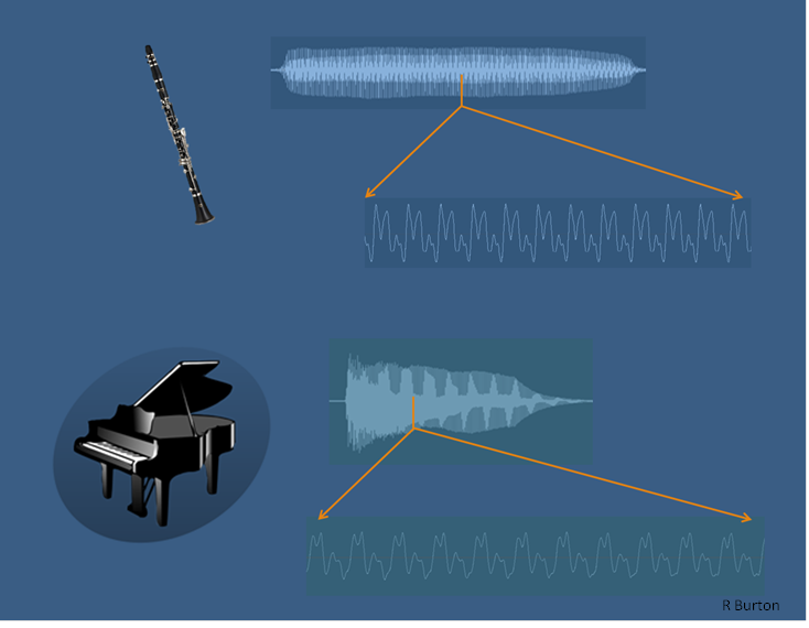
*By Rburtonresearch - Own work, CC BY-SA 4.0,
https://commons.wikimedia.org/w/index.php?curid=45074868 -
Texture: the composition of multiple sounds into a single perceived moment of noise, whether harmonized into music or a dissonant cacophony of overlapping sounds.
-
Location: the location of the source of the sound with respect to the listener's environment.
Each of these qualities are affected by different aspects of the sound wave like its frequency, amplitude, or shape. When we go to synthesize our own music, we will be able to control the actual waves our speakers generate. This will enable us to completely control all of these different qualities of the music we produce.
MIDI and Scamper
Further in the course, we will generate our own sounds. But for now, we
are going to limit our interactions to the MIDI interface in the Scamper
music library. The timbre of the MIDI music is mostly fixed (except
for a few mods like the percussion mod), but the other sound qualities
can be controlled through several functions or specified values.
The Pitch of a note is specified by the given MIDI value, which is an integer from 0 to 127. Each of these integers refers to a note in the classical western tradition. Some important note values are 60 (Middle-C, C4, 261.63 Hz) and 69 (A4, Concert Pitch, 440 Hz). The MIDI values from 21 to 108 are the keys on the classical piano.
The Duration of a note can be controlled with dur. We will explore
this in much more detail in the future. For now, it is useful to know
there are a number of specified values. Two important ones are qn
denoting a quarter note (a standard 'beat'), and en denoting an eighth
note (half of a standard 'beat').
The Loudness of a note can be controlled through the use of mod and
dynamics functions. We'll see examples in lab.
The mod and percussion functions can be used to have notes represent
specific percussive instruments.
Harmonics
In this reading, we are going to explore the concept of Pitch and further examine how changing the pitch of notes can alter the resulting music we produce.
Subdividing a String
First recall that we defined musical tones as vibrations in the air (typically), and that our reference note for concert pitch was A4, which vibrates with a frequency of 440 Hz (440 high pressure peaks per second). We are going to start with this pitch, and use a simple thought experiment to begin deriving other pitches!
Let's consider a specific example of producing this sound: plucking a string that vibrates at exactly 440 Hz:
(Credit: Juan M. Aguirregabiria author of Easy Java Simulation = Francisco Esquembre, CC BY-SA 3.0 https://creativecommons.org/licenses/by-sa/3.0, via Wikimedia Commons)
Now clearly this animation is not vibrating at 440 Hz (since that would be a bit too fast to easily see the motion), but it demonstrates the motion of the vibrating string.
We should note that this figure shows one possible way the string can vibrate when plucked. What is shown is the most natural mode of vibration, what we call the resonant frequency, where the full string sways back-and-forth together. But there are actually other modes of vibration. If we add a fixed point in the middle of the string, we can see that vibrations can form with a wave of half the wavelength (related to the distance between the fixed points) as the previous vibration. Halving the wavelength results in doubling the frequency of the produced pitch.
(Credit: Juan M. Aguirregabiria author of Easy Java Simulation = Francisco Esquembre, CC BY-SA 3.0 https://creativecommons.org/licenses/by-sa/3.0, via Wikimedia Commons)
But what is the affect of doubling the frequency on the pitch produced? What new tone have we developed?
If we start with A4 at 440 Hz, doubling the frequency gives us 880 Hz, which we label as A5. Here's the two played together:
(import music)
(seq (note 69 qn) (rest en)
(note 81 qn) (rest en)
(par (note 69 qn) (note 81 qn)))
Somehow, our brains recognize these as the same note, just one is higher up than the other! That's why we give them both the label A. We can keep doubling (or halving) to produce other As as well, they go from A0 at 27.5 Hz (the lowest note on the piano) to A7 at 3520 Hz (a little lower than the upper note on the piano, which is C8 at 4186.01 Hz).
Of course, you can continue going up or down in either direction, human hearing just has trouble keeping up. Each time we double or halve the frequency, we say we have moved up or down an octave: A5 is one octave above A4.
The Overtone Series
So we can halve the mode to go up an octave, but what if we try something like dividing our string into three vibrating sections (with 2 fixed points in the interior)? We get a brand new note as 3 times the frequency of the original note!

*Lookang many thanks to author of original simulation = Juan M. Aguirregabiria author of Easy Java Simulation = Francisco Esquembre, CC BY-SA 3.0 https://creativecommons.org/licenses/by-sa/3.0, via Wikimedia Commons
So what is this new note at 440*3=1320 Hz? It doesn't quite exist in modern western music. It turns out that some of the arithmetic gets weird when we keep going with our subdivisions of the string, and to deal with it, western music settled on a standard tuning that adjusts everything slightly to make the numbers mostly align.
Instead of exactly 3 times the original frequency for A4 (which should be 1320 Hz), we define E6 as 1318.51. It's pretty close at least! Let's listen to these notes together:
(import music)
(seq (note 69 qn) (rest en)
(note 81 qn) (rest en)
(note 88 qn) (rest en)
(par (note 69 qn) (note 81 qn) (note 88 qn)))
They sound pretty good together, though that new note is definitely a distinct new pitch.
Here's an interesting question to ask: what if we take our new E6 and halve its frequency to get what we might call E5? This totally works, and gives us E5, a note with a adjusted frequency set at 659.26 Hz.
What is the relationship between this new E5 and the original A4? We tripled the frequency to get to E6, then halved it to get to E5, so we have a new frequency of 3/2 of the original frequency:
440 Hz * 3/2 = 660 Hz ~ 659.26 Hz (E5)
Let's hear these notes together:
(import music)
(seq (note 69 qn) (rest en)
(note 76 qn) (rest en)
(note 81 qn) (rest en)
(note 88 qn) (rest en)
(par (note 69 qn) (note 76 qn)) (rest en)
(par (note 81 qn) (note 88 qn)))
But why stop at subdividing 3 times, what if we subdivide 4 times (~A6), or 5 times (~C#7), or more? This is called the overtone series!
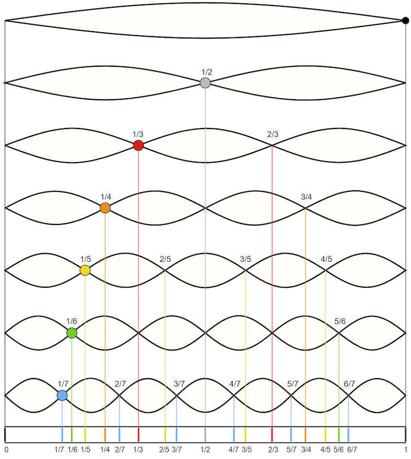
*By Moodswingerscale.jpg: Y Landmanderivative work: W axell, Public domain, via Wikimedia Commons
The Western Chromatic Scale
If we continue this process of subdivision, and follow what the western musicians eventually settled on as a standard tuning, you end up with 12 roughly equally spaced notes in a single octave. Below is code that will play these notes for the octave between A4 and A5. This code plays the 12 notes and arrives back at the 13th (the repeated full octave). The names of the notes are provided as comments (some notes have two names, with # pronounced "sharp" and b pronounced "flat").
(import music)
(seq (note 69 qn) (rest en) ; A4
(note 70 qn) (rest en) ; A#4 / Bb4
(note 71 qn) (rest en) ; B4
(note 72 qn) (rest en) ; C5
(note 73 qn) (rest en) ; C#5 / Db5
(note 74 qn) (rest en) ; D5
(note 75 qn) (rest en) ; D#5 / Eb5
(note 76 qn) (rest en) ; E5
(note 77 qn) (rest en) ; F5
(note 78 qn) (rest en) ; F#5 / Gb5
(note 79 qn) (rest en) ; G5
(note 80 qn) (rest en) ; G#5 / Ab5
(note 81 qn) (rest en)) ; A5
This sequence is called "the chromatic scale."
Western music is commonly composed by first choosing certain specified subset of these possible chromatic notes and composing music while remaining mostly limited to those notes and the chords that they can produce. We call that type of subset of chromatic notes a 'scale.'
The most common scale in the western tradition is the Major Scale. Below is the subset of our chromatic notes in sequence which produce the A-Major Scale:
(import music)
(seq (note 69 qn) (rest en) ; A4
(note 71 qn) (rest en) ; B4
(note 73 qn) (rest en) ; C#5 / Db5
(note 74 qn) (rest en) ; D5
(note 76 qn) (rest en) ; E5
(note 78 qn) (rest en) ; F#5 / Gb5
(note 80 qn) (rest en) ; G#5 / Ab5
(note 81 qn) (rest en)) ; A5
We'll return to this discussion of scales in the future, and explore the western rules of selecting notes to form a scale. These rules are based on the relationship between the frequency of the notes selected. The notes picked for each scale are related to important overtones of the root note of the scale.
Of course, some non-western traditions will require a return to our previous discussion of frequencies and further subdividing of our vibrating string...
Lab: Scales and Chords
In today's lab, we'll look at the relationship between pitches by writing code that generates scales and chords.
Additionally, we'll examine the section and compose/o operations in more detail.
and follow the instructions.
When you are done, make sure to save the file and then upload the completed lab to Gradescope.
Transforming RGB colors
We examine the building blocks of one of the common kinds of algorithms used for RGB colors: Generating new colors from existing colors.
Introduction
We have just started to learn about RGB colors, and so the operations we might do on images and colors are somewhat basic. How will we expand what we can do, and what we can write? In part, we will learn new Scheme techniques, applicable not just to image computation, but to any computation. In part, we will learn new functions in Scamper that support more complex image computations. In part, we will write our own more complex functions.
For now, we will focus on transforming color images. One common algorithmic approach to images is the construction of
In readings and labs, we will consider filters that are constructed by transforming each color in an image using an algorithm that converts one RGB color to another. In this reading, as well as some followups, we will consider some basic approaches for transforming images, including some basic operations for transforming colors and ways to combine them into more complex transformations.
Some basic transformations
Rather than writing every transformation from scratch, we will start with a few basic transformations in the image library.
Making colors lighter and darker
The simplest transformations are rgb-darker and rgb-lighter. These operations make a color a little bit darker and a little bit lighter. If you apply them repeatedly, you can darker and darker (or lighter and lighter) colors, eventually reaching black (or white).
> (color-name->rgb "blueviolet")

> (rgb->string (color-name->rgb "blueviolet"))
"138/43/226"
> (rgb-darker (color-name->rgb "blueviolet"))

> (rgb->string (rgb-darker (color-name->rgb "blueviolet")))
"122/27/210"
> (rgb-darker (rgb-darker (color-name->rgb "blueviolet")))

> (rgb->string (rgb-darker (rgb-darker (color-name->rgb "blueviolet"))))
"106/11/194"
> (rgb-lighter (color-name->rgb "blueviolet"))

> (rgb->string (rgb-lighter (color-name->rgb "blueviolet")))
"154/59/242"
Note that these are pure procedures. When you compute a darker or lighter version of a color, the purpose is to create a new color. Hence, the original color is unchanged.
Transforming components
In addition to making the color uniformly darker or lighter, we can also
increase individual components using rgb-redder, rgb-greener, and
rgb-bluer.
> (color-name->rgb "blueviolet")
> (rgb->string (color-name->rgb "blueviolet"))
"138/43/226"
> (rgb-redder (color-name->rgb "blueviolet"))

> (rgb-greener (color-name->rgb "blueviolet"))

> (rgb-bluer (color-name->rgb "blueviolet"))

> (rgb->string (rgb-redder (color-name->rgb "blueviolet")))
"170/27/210"
> (rgb->string (rgb-greener (color-name->rgb "blueviolet")))
"122/75/210"
> (rgb->string (rgb-bluer (color-name->rgb "blueviolet")))
"122/27/255"
As the examples suggest, for some people, making a color slightly redder, greener, or bluer is hard to detect. Sometimes it's easier to see the changes if we make the transformations a few times. (Since the first call to rgb-bluer increases the blue component to its largest value, we may not see further increases.)
> (rgb-redder (rgb-redder (color-name->rgb "blueviolet")))

> (rgb-greener (rgb-greener (color-name->rgb "blueviolet")))

> (rgb-bluer (rgb-bluer (color-name->rgb "blueviolet")))

> (rgb->string (rgb-redder (rgb-redder (color-name->rgb "blueviolet"))))
"202/11/194"
> (rgb->string (rgb-greener (rgb-greener (color-name->rgb "blueviolet"))))
"106/107/194"
> (rgb->string (rgb-bluer (rgb-bluer (color-name->rgb "blueviolet"))))
"106/11/255"
Other simple transformations
The rgb-rotate procedure rotates the red, green, and blue components of a color, setting red to green, green to blue, and blue to red. It is intended mostly for fun, but it can also help us think about the use of these components.
> (color-name->rgb "blueviolet")
> (rgb->string (color-name->rgb "blueviolet"))
"138/43/226"
> (rgb-rotate-components (color-name->rgb "blueviolet"))

> (rgb->string (rgb-rotate-components (color-name->rgb "blueviolet")))
"43/226/138"
> (rgb-rotate-components (rgb-rotate-components (color-name->rgb "blueviolet")))

> (rgb->string (rgb-rotate-components (rgb-rotate-components (color-name->rgb "blueviolet"))))
"226/138/43"
The rgb-phaseshift procedure is another procedure with less clear uses. It adds 128 to each component with a value less than 128 and subtracts 128 from each component with a value of 128 or more. While this is somewhat like the computation of a pseudo-complement, it also differs in some ways. Hence, the image library also provides a rgb-pseudo-complement procedure that computes the pseudo-complement of an RGB color.
> (color-name->rgb "blueviolet")
> (rgb->string (color-name->rgb "blueviolet"))
"138/43/226"
> (rgb-phaseshift (color-name->rgb "blueviolet"))

> (rgb->string (rgb-phaseshift (color-name->rgb "blueviolet")))
"10/171/98"
> (rgb-pseudo-complement (color-name->rgb "blueviolet"))

> (rgb->string (rgb-pseudo-complement (color-name->rgb "blueviolet")))
"117/212/29"
Writing your own color transformations
At the beginning of this reading, you learned a few basic procedures for transforming colors. Are these the only ways that you can transform colors? Certainly not! You are free to write your own color transformations. For example, you might decide that rgb-greener should use a more complicated formula for making colors greener, scaling multiplicatively rather than additively.
(define greener
(lambda (c)
(rgb (* 9/10 (rgb-red c))
(+ 8 (* 11/10 (rgb-green c)))
(* 9/10 (rgb-blue c))
(rgb-alpha c))))
Let's see how well that works.
> (color-name->rgb "blueviolet")
> (greener (color-name->rgb "blueviolet"))

> (greener (greener (color-name->rgb "blueviolet")))

> (greener (greener (greener (color-name->rgb "blueviolet"))))

> (greener (greener (greener (greener (color-name->rgb "blueviolet")))))

> (greener (greener (greener (greener (greener (color-name->rgb "blueviolet"))))))

> (rgb->string (color-name->rgb "blueviolet"))
"138/43/226"
> (rgb->string (greener (color-name->rgb "blueviolet")))
"124/55/203"
> (rgb->string (greener (greener (color-name->rgb "blueviolet"))))
"112/68/183"
> (rgb->string (greener (greener (greener (color-name->rgb "blueviolet")))))
"101/83/165"
> (rgb->string (greener (greener (greener (greener (color-name->rgb "blueviolet"))))))
"91/99/148"
Of course, this is not the only way to define a procedure like greener. We could also define it in terms of the existing procedures. For example, since rgb-greener seems to increment the green component by 32 and rgb-darker seems to decrement all three components by 16, we could try something like
(define greener2
(lambda (c)
(rgb-greener (rgb-greener (rgb-darker (rgb-darker c))))))
> (color-name->rgb "blueviolet")
> (rgb->string (color-name->rgb "blueviolet"))
"138/43/226"
> (greener2 (color-name->rgb "blueviolet"))

> (rgb->string (greener2 (color-name->rgb "blueviolet")))
"74/75/162"
There are also color transformations you cannot build (at least not easily) from the basic transformation. For example, suppose you want to eliminate extreme colors. You might choose to bound each component so that it is at least 64 and no more than 192.
;;; (bound val lower upper) -> number?
;;; val : number?
;;; lower : number?
;;; upper : number?
;;; "Bounds" `val`, ensuring that the result is `lower` if `val` is
;;; less than `lower` and `upper` if `val` is greater than `upper`.
(define bound
(lambda (val lower upper)
(max lower (min upper val))))
;;; (bound-component component) -> integer?
;;; component : integer?
;;; Bounds a component to a value between 64 and 192.
(define bound-component
(lambda (component)
(bound component 64 192)))
;;; (rgb-bound c) -> rgb?
;;; c : rgb?
;;; Bound all of the components of `c`.
(define rgb-bound
(lambda (c)
(rgb (bound-component (rgb-red c))
(bound-component (rgb-green c))
(bound-component (rgb-blue c))
(rgb-alpha c))))
Let's try it out.
> (color-name->rgb "blueviolet")
> (rgb->string (color-name->rgb "blueviolet"))
"138/43/226"
> (rgb-bound (color-name->rgb "blueviolet"))

> (rgb->string (rgb-bound (color-name->rgb "blueviolet")))
"138/64/192"
> (color-name->rgb "black")

> (rgb->string (color-name->rgb "black"))
"0/0/0"
> (rgb-bound (color-name->rgb "black"))

> (rgb->string (rgb-bound (color-name->rgb "black")))
"64/64/64"
> (color-name->rgb "whitesmoke")

> (rgb->string (color-name->rgb "whitesmoke"))
"245/245/245"
> (rgb-bound (color-name->rgb "whitesmoke"))

> (rgb->string (rgb-bound (color-name->rgb "whitesmoke")))
"192/192/192"
Self checks
Check 1: Repeated transformations
We've seen that applying rgb-darker multiple times makes a color much darker. What do you expect to happen if we apply each of the following two times?
rgb-boundrgb-pseudo-complementrgb-phaseshift
Check 2: Inverse transformations (‡)
rgb-lighter and rgb-darker seem to be inverses of each other. That is, if we make a color darker and then lighter, we seem to end up with the same color.
> (rgb-darker (rgb-lighter (rgb 100 100 100)))

> (rgb->string (rgb-darker (rgb-lighter (rgb 100 100 100))))
"100/100/100"
Are there any colors for which (rgb-darker (rgb-lighter c)) gives a different color?
Check 3: Writing new transformations
Write a procedure, (rgb-grey c), that takes an RGB color as input and produces a greyscale color, one in which the red, green, and blue components are the same (and equal to the average of the components in c).
Transforming images
We explore how to expand the power of color transformations, first by applying them to images rather than to individual colors then by further combining them into new transformations.
From transforming colors to transforming images
You may have been asking why we have been focusing on transforming individual colors, other than that using the transformations helps us better understand the underlying representation. Here's one reason: Many image filters are written by applying a transformation to each color in the image.
So, how do we write image filters? That is, how do we generalize color transformations to image filters? The csc151 library includes a helpful procedure, (pixel-map colortrans image), that builds a new image by setting the color at each position in the new image to the result of applying the given color transformation to the color at the corresponding position in the original image.
Using pixel-map and the color transformations we learned in the previous reading, we can now transform images in a few basic ways: we can lighten images, darken images, complement images (and perhaps even compliment the resulting images), and so on and so forth.
Let's consider a few examples. We'll start with this public domain image of a kitten, which we will refer to as kitten.
This image can be loaded via the with-image-from-url function.
(with-image-from-url url fn) takes two arguments:
- The uniform resource locator, i.e., URL, of an image. URLs are used to specify the location of a file on the internet.
- A callback function
fnthat takes the image Scamper loads from the URL as input. The output offnis then rendered to the output pane.
The URL of the kitten image is:
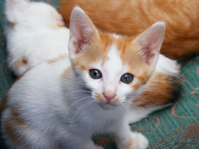
(Note: For security reasons related to running within a web browser, Scamper currently cannot load images not found on scamper.cs.grinnell.edu!)
For example, here are two uses of the function.
The first use simply outputs the image unmodified.
The second applies a transformation via pixel-map.
(with-image-from-url "https://scamper.cs.grinnell.edu/images/kitten.jpg"
(lambda (img)
img))

(with-image-from-url "https://scamper.cs.grinnell.edu/images/kitten.jpg"
(lambda (img)
(pixel-map rgb-redder img)))
Composing transformations
But what if we want more interesting filters, ones that can't be described with just a single built-in transformation? One thing that we can do is to combine transformations. There are two ways to transform an image using more than one transformation: You can do each transformation in sequence, or you can use function composition, an old mathematical trick that you learned how to do in Scheme in the last reading. Consider, for example, the problem of lightening an image and then increasing the red component. We can certainly write the following sequence of definitions.
> (define intermediate-picture (pixel-map rgb-redder picture))
> (define modified-picture (pixel-map rgb-darker intermediate-picture))
However, it is not necessary to name the intermediate image. We can instead choose to nest the calls to pixel-map, using something like this definition.
> (define modified-picture (pixel-map rgb-darker (pixel-map rgb-redder picture)))
However, even this more concise instruction still creates the intermediate (redder but not lighter) version of the picture. Can we make each color in the image both redder and lighter?
In a recent reading, we learned that we can define a new transformation by combining other transformations with the composition function, compose (or its shorthand, o). Using that function, we can write the following instructions.
> (define rgb-fun (o rgb-lighter rgb-redder))
> (define modified-picture (pixel-map rgb-fun picture))
But even that is a bit verbose. Do we really want to name rgb-fun when we only use it once? No. Fortunately, Scheme lets us use the function created by compose without naming it, just as it lets us use most expressions without naming them.
> (define modified-picture (pixel-map (o rgb-darker rgb-redder) picture))
Let's try this on our kitten.
(with-image-from-url "https://scamper.cs.grinnell.edu/images/kitten.jpg"
(lambda (img)
(pixel-map (o rgb-darker rgb-redder) kitten)))
What's the difference between this instruction and the nested calls to pixel-map? In effect, we've changed the way you sequence operations. That is, rather than having to write multiple instructions, in sequence, to get something done, we can instead insert information about the sequencing into a single instruction. By using composition, along with nesting, we can then express our algorithms more concisely and often more clearly. It is also likely to be a bit more efficient, since we make one new image, rather than two.
Detour: Saving images
It's useful to be able to load images so that we can manipulate them. It's even more useful to be able to save images that we've created. Luckily, since Scamper operates in the browser, the images we see in the output are genuine images that we simply download! To download an image that you create, right-click on the image and select "Save image as..." (or the equivalent in your browser).
Mapping binary color procedures with section
So far, so good. We know how to load images with image-load. We know how to make new versions of existing images using pixel-map. We know how to save the result using image-save. Are we missing anything?
It turns out that we're missing a few things. Right now, the only way we can make a variant of an image is using one of the unary (single-parameter) procedures, either the built-in procedures, such as rgb-redder, or ones we create with the composition operator, compose. But we know other procedures transforming colors, such as rgb-subtract or rgb-average, that are not unary. (In case you haven't encountered these procedures, you can find them at the end of the reading.) How do we use such procedures?
It doesn't make sense to write (rgb-subtract pic (rgb 0 0 255)), since picture is not an RGB color. Hopefully, we'll get an error message if we try.
> (with-image-from-url "https://scamper.cs.grinnell.edu/images/kitten.jpg"
(lambda (img)
(rgb-subtract img (rgb 0 0 255))))
Runtime error [10:5-10:36]: (rgb-subtract) expected an RGB value, received object
It also doesn't make sense to use rgb-subtract as the first parameter to pixel-map, as in (pixel-map rgb-subtract pic), because we don't have a place to specify the color we are subtracting. Once again, Scamper should issue an error message.
> (with-image-from-url "https://scamper.cs.grinnell.edu/images/kitten.jpg"
(lambda (img)
(pixel-map rgb-subtract img))
Runtime error [8:5-8:32]: (pixel-map) wrong number of arguments to rgb-subtract provided. Expected 2, received 1.
Not the most helpful error message, but an error message nonetheless.
We might be tempted to write something like (pixel-map pic (rgb-subtract (rgb 0 0 255)). However, that will also cause problems, since it looks like we are calling rgb-subtract on a single value, and not the two values it is supposed to take.
> (with-image-from-url "https://scamper.cs.grinnell.edu/images/kitten.jpg"
(lambda (img)
(pixel-map (rgb-subtract (rgb 0 0 255)) img)))
Runtime error [8:16-8:43]: (rgb-subtract) wrong number of arguments to rgb-subtract provided. Expected 2, received 1.
It's probably good that we get an error message here, since it's not clear whether (rgb 0 0 255) is supposed to be the first or second parameter to rgb-subtract---are we subtracting (rgb 0 0 255) from each color, or are we subtracting each color from (rgb 0 0 255)?
To handle situations like this, scamper includes a special form, section, that lets you fill in some parameters to a function. It takes the form (section procedure arg1 arg2 ...)). In other words the syntax is like a function call (procedure arg1 arg2 ...) except with section at the front!
When we want to fill in a particular parameter, we write the value we want. When we want to leave a parameter blank, we write the special symbol _. For example, here's a function that subtracts the blue component from every color.
(define rgb-subtract-blue (section rgb-subtract _ (rgb 0 0 255)))
(with-image-from-url "https://scamper.cs.grinnell.edu/images/kitten.jpg"
(lambda (img)
(pixel-map rgb-subtract-blue img)))
If, instead, we want to subtract the current color from white (which is how we computed the pseudo-complement), we can swap the place that we put the special symbol.
(define rgb-subtract-from-white (section rgb-subtract (rgb 255 255 255) _))
(with-image-from-url "https://scamper.cs.grinnell.edu/images/kitten.jpg"
(lambda (img)
(pixel-map rgb-subtract-from-white img)))

As in the case of unary functions created with compose, we don't have to name the function we create. Here's an instruction that will make a somewhat bluer version of the kitten.
(with-image-from-url "https://scamper.cs.grinnell.edu/images/kitten.jpg"
(lambda (img)
(pixel-map (section rgb-average (rgb 0 0 255) _)
img)))

Self checks
Check 1: Fade to grey
a. Without using a lambda, write a procedure, (average-with-grey c), that everages c with (rgb 127 127 127).
b. What do you expect to happen if you transform the image with average-with-grey?
c. Check your answer experimentally.
d. What do you expect to happen if you twice transform the image with average-with-grey?
e. Check your answer experimentally.
Binary RGB procedures
Here are the binary RGB procedures mentioned above in the discussion of cutting.
;;; (rgb-subtract c1 c2) -> rgb?
;;; c1 : rgb?
;;; c2 : rgb?
;;; Create a new RGB color by subtracting each component of `c2` from
;;; the corresponding component of `c1`.
(define rgb-subtract
(lambda (c1 c2)
(rgb (- (rgb-red c1) (rgb-red c2))
(- (rgb-green c1) (rgb-green c2))
(- (rgb-blue c1) (rgb-blue c2))
(rgb-alpha c1))))
;;; (rgb-average c1 c2) -> rgb?
;;; c1 : rgb?
;;; c2 : rgb?
;;; Create a new RGB color by averaging the corresponding components of
;;; c1 and c2.
(define rgb-average
(lambda (c1 c2)
(rgb (* 1/2 (+ (rgb-red c1) (rgb-red c2)))
(* 1/2 (+ (rgb-green c1) (rgb-green c2)))
(* 1/2 (+ (rgb-blue c1) (rgb-blue c2)))
(* 1/2 (+ (rgb-alpha c1) (rgb-alpha c2))))))
Transforming images
We explore techniques for transforming images, focusing on the use of anonymous procedures.
Procedures to remember
Basic color procedures
(rgb r g b)- create a new RGB color.(rgb r g b a)- create a new RGB color, also specifying the alpha channel.(rgb-red c)- extract the red component of an rgb color.(rgb-green c)- extract the green component of an rgb color.(rgb-blue c)- extract the blue component of an rgb color.
Transforming colors
(rgb-darker c)- create a darker version ofc(if possible).(rgb-ligheter c)- create a lighter version ofc(if possible).(rgb-redder c)- create a redder version ofc(if possible).(rgb-greener c)- create a greener version ofc(if possible).(rgb-bluer c)- create a bluer version ofc(if possible).(rgb-pseudo-complement c)- get the pseudo-complement ofc.(rgb-complement c)- get the HSV complement ofc.(rgb-greyscale c)- convert c to greysacle.(rgb-phaseshift c)- phase shift each component ofcby 128, adding 128 to values less than 128 and subtracting 128 from values greater than or equal to 128.(rgb-rotate-components c)- rotate the RGB components ofc.
Combining colors
(rgb-add c1 c2)- Add the components of two RGB colors.(rgb-subtract c1 c2)- Subtract corresponding components ofc2fromc1.(rgb-average c1 c2)- Average the components inc1andc2.
Working with color names
(all-color-names)- list all the color names.(color-name->rgb name)- convert a color name to an RGB color.(find-colors name)- find all the colors that include name.
Working with images
(with-image-file fn)- loads an image, callingfnwith the image as input.(with-image-from-url url fn)- loads an image fromurl, callingfnon the image as input.(pixel-map color-transformation image)- apply a color transformation to each pixel in an image.- `(image-save img filename) - save an image to a file.
Working with procedures
(section (expression-with-underscores))- Build a new procedure that takes one parameter for each underscore inexpression-with-underscores.(o fun1 fun2 fun3 ... funk)- Build a new procedure that appliesfunkthen ... thenfun3thenfun2thenfun1to its parameter.
The lab
- Use the file transforming-images.scm.
- Find an image you like, such as your campus directory picture (or President Harris' directory picture, or your instructor's directory picture) and save it to your desktop.
Acknowledgements
The kitten image was downloaded from http://public-photo.net/displayimage-2485.html. Unfortunately, the site behind that URL has disappeared. Nonetheless, the kitten image lives on.
This lab was originally written in 2024Sp, based on a lab from 2017Sp.
Naming values with local bindings
Algorithm designers regularly find it useful to name the values their algorithms process. We consider why and how to name new values that are only available within a procedure.
Introduction
When writing programs and algorithms, it is useful to name values we compute along the way. For example, in an algorithm that, given a list of numbers, sorts that list of numbers, it may be useful to name the sorted list along the way. When we associate a name with a value, we say that we bind that name to the value.
So far we've seen three ways in which names are bound to values in Scheme.
- The names of built-in procedures, such as
+andquotient, are predefined. There are also some predefined values, such aspi. When the Scheme interpreter starts up, these names are already bound to the procedures they denote. - The programmer can introduce a new binding by means of a definition. A definition may introduce a new equivalent for an old name, or it may give a name to a newly computed value.
- When a programmer-defined procedure is called, the parameters of the procedure are bound to the values of the corresponding arguments in the procedure call. Unlike the other two kinds of bindings, parameter bindings are local -- they apply only within the body of the procedure. Scheme discards these bindings when it leaves the procedure and returns to the point at which the procedure was called.
As you develop more and longer procedures, you will find that there are many times you want to create local names for values that are not parameters. We will consider such names in this reading.
Redundant work
You will find that there are many times when you are designing algorithms that you end up telling the computer to do the same thing again and again and again. For example, here's a bit of code that determines the ratio of vowels to consonants and let's see how well it works.
;;; (tally f l) -> number?
;;; f : function?, a predicate over elements of l
;;; l : list?
;;; Returns the number of occurrences that f returns
;;; #t for each element of the list.
(define tally
(lambda (f l)
(if (null? l)
0
(+ (if (f (car l))
1
0)
(tally f (cdr l))))))
;;; (vowel? ch) -> boolean?
;;; ch : char?
;;; Determine whether ch is a vowel.
(define vowel?
(lambda (ch)
(or (char=? (char-downcase ch) #\a)
(char=? (char-downcase ch) #\e)
(char=? (char-downcase ch) #\i)
(char=? (char-downcase ch) #\o)
(char=? (char-downcase ch) #\u))))
;;; (consonant? ch) -> boolean?
;;; ch : char
;;; Determine if ch is a consonant
(define consonant?
(lambda (ch)
(and (char-alphabetic? ch) (not (vowel? ch)))))
;;; (v2c-ratio str) -> rational?
;;; str : string
;;; Determine the ratio of vowels to consonants in str
(define v2c-ratio
(lambda (str)
(/ (tally vowel? (string->list str))
(tally consonant? (string->list str)))))
(v2c-ratio "Hello")
(v2c-ratio "Aaargh!")
(v2c-ratio "aeiouxy")
; Whoops!
(v2c-ratio "a")
'Eh. It's good enough for now.
But there's a problem with the design. We're repeating some work.
Please identify some points at which we repeat work.
We mean it.
That is, stop here and ask yourself, "Where does the code duplicate work?"
Are you done?
Are you sick of these pauses? If more students paused when we asked questions, we wouldn't have to insert these kinds of notes.
Anyway, work is being repeated in at least three ways.
- First, we call
(char-downcase ch)as many as five times. It feels like we should be able to do it once. - Second, we call
(string->list str)twice. It feels like we should be able to do it once. This may even have a bigger effect than the five calls tochar-downcasebecause building lists can be "expensive". - Third, we ask if many letters are a vowel twice, once when counting the vowels and once when counting the consonants.
That last problem is going to be hard to deal with, particularly as we
try to keep our code readable. So let's focus on the first two. Can
we avoid calling (char-downcase ch) so many times?
Yes, you can fill in the annoying delay now.
Here's one approach: We can decompose the task into two tasks. We'll write one procedure that determines if a character is a lowercase vowel.
;;; (lower-case-vowel? ch) -> boolean?
;;; ch : char?
;;; Determine whether ch is a lowercase vowel.
(define lower-case-vowel?
(lambda (ch)
(or (char=? ch #\a)
(char=? ch #\e)
(char=? ch #\i)
(char=? ch #\o)
(char=? ch #\u))))
That seems straightforward enough, doesn't it? Our vowel? procedure
can then call that other procedure using a letter converted to lowercase.
;;; (vowel? ch) -> boolean?
;;; ch : char?
;;; Determine whether ch is a vowel.
(define vowel?
(lambda (ch)
(lower-case-vowel? (char-downcase ch))))
About as easy to read as before. A little more typing on our part. And we've saved some computation. In fact, this kind of decomposition is a strategy programmers use fairly frequently: Rewrite procedures that do a sequence of steps by using one procedure for each step.
In fact, now that we've phrased it as a sequence of steps, we can take advantage of composition.
;;; (vowel? ch) -> boolean? ;;; ch : char? ;;; Determine whether ch is a vowel. (define vowel? (o lower-case-vowel? char-downcase))
Detour: Why are we repeating the documentation each time we show
you a new imlementation of the vowel? predicate? Mostly to
remind you that there's a value to writing documentation, even
when our procedures are short and simple.
Will anyone ever use lower-case-vowel? by itself? Possibly.
But if not, we should try something else. Is there something
else?
Racket's let Expressions
There is. Racket provides let expressions as a way to bind
values to names. A let-expression contains a binding list and
a body. The body can be any expression, or any sequence of
expressions, to be evaluated with the help of the local name bindings.
The binding list takes the form of a parentheses enclosing zero or
more binding expressions of the form (name value).
That precise definition may have been a bit confusing, so here's the
general form of a let expression
(let ([name1 exp1]
[name2 exp2]
...
[namen expn])
body
As shorthand, we call each of the name-expression pairs of a
let-expression a binder.
When the Racket evaluator encounters a let-expression, it begins
by evaluating all of the expressions inside its binding specifications.
Then the names in the binding specifications are bound to those
values. Next, the expressions making up the body of the let-expression
are evaluated, in order. The value of the last expression in the
body becomes the value of the entire let-expression. Finally, the
local bindings of the names are cancelled. (Names that were unbound
before the let-expression become unbound again; names that had
different bindings before the let-expression resume those earlier
bindings.)
What do we mean by "bound"? As you may recall, the Racket evaluator maintains a table of names and corresponding values. We call that association a "binding". When the evaluator encounters a name, it looks up the binding in the table.
Here's one way to write vowel? with let and
without helpers.
;;; (vowel? ch) -> boolean?
;;; ch : char?
;;; Determine whether ch is a vowel.
(define vowel?
(lambda (ch)
(let ([lc (char-downcase ch)])
(or (char=? lc #\a)
(char=? lc #\e)
(char=? lc #\i)
(char=? lc #\o)
(char=? lc #\u)))))
Important! Note that even though binding lists and binding
specifications start with parentheses, they are not procedure
calls; their role in a let-expression simply to give names to
certain values while the body of the expression is being evaluated.
The outer parentheses in a binding list are structural -- they are
there to group the pieces of the binding list together.
As we've seen, using a let-expression often simplifies an expression
that contains two or more occurrences of the same subexpression.
The programmer can compute the value of the subexpression just once,
bind a name to it, and then use that name whenever the value is
needed again. Sometimes this speeds things up by avoiding such
redundancies as the recomputation of values. In other cases, there
is little difference in speed, but the code may be a little clearer.
Comparing let and define
You may have missed it, but there are a few subtle and important
issues with the use of let rather than define to name values
and procedures. One difference has to do with the availability
(or scope) of the name. Values named by define are available
essentially everywhere in your program. In contrast, values named by
let are available only within the let expression. (In case you were
wondering, the term scope has nothing to do with the mouthwash.)
In addition, local variables (given by let) and global variables (given by our
standard use of define) affect previous uses of the name differently (or at
least appear to). When we do a new top-level define, we permanently replace
the old value associated with the name. That value is no longer accessible. In
contrast, when we use let to override the value associated with a name, as
soon as the let binding is finished, the previous association is restored.
Finally, there's a benefit to using let instead of define according to
the principle of information hiding. Evidence suggests that programs
work better if the various pieces do not access values relevant primarily
to the internal workings of other pieces. If you use define for your
names, they are accessible (and therefore modifiable) everywhere. Hence,
you enforce this separation by policy or obscurity. In contrast, if
you use let to define your local names, these names are completely
inaccessible to other pieces of code. We return to this issue in our
discussion of the ordering of let and lambda below.
Our mental model of computation and let
Now that we've discussed how let works at a high-level, let's consider how let behaves precisely within the context of our mental model of computation.
For example, consider the following expression:
(let ([x (+ 1 1)]
[y (* 2 3)]
[z (- 8 5)])
(+ x y z))
We think about evaluating a let-expression in multiple stages.
- First, we evaluate the expression of each binding of the
letto values. - We then (a) substitute the resulting value for the binder's corresponding variable everywhere that variable occurs in the body of the
letand (b) substitute the body of theletfor the overalllet-expression. - Finally, we continue evaluating the substituted
let-body as normal.
Let's see how this works in our example above.
First, we must evaluate each of the binding expressions in turn:
(let ([x (+ 1 1)]
[y (* 2 3)]
[z (- 8 5)])
(+ x y z))
--> (let ([x 2]
[y (* 2 3)]
[z (- 8 5)])
(+ x y z))
--> (let ([x 2]
[y 6]
[z (- 8 5)])
(+ x y z))
--> (let ([x 2]
[y 6]
[z 3])
(+ x y z))
Now, we must substitute values-of-bound-variables in the body of the let and then substitute the let-body itself.
From the above expression, we will substitute 2 for x, 6 for y, and 3 for z everywhere in the expression (+ x y z).
The resulting expression is what the entire let evaluates to.
From there, we evaluate the expression normally to arrive at a final result.
--> (let ([x 2]
[y 6]
[z 3])
(+ x y z))
--> (+ 2 6 3)
--> 11
Note that we only substitute for the variable as it appears in the body of the let.
We do not substitute for the variable if it occurs outside of the body!
For example, if we nest a let-binding in larger computation:
(+ (let ([x 1])
(* x 5))
(- x 1))
There are two occurrences of x here:
(* x 5): this is the body of theletso we will eventually substitute1for it.(- x 1): this is the second argument to+and is outside the body of thelet, so we do not substitute for it. Presumably, thisxis bound by a different construct, e.g., adefine.
Sequencing bindings with let*
Sometimes we may want to name a number of interrelated things. For
example, suppose we wanted to square the average of a list of numbers.
(It may not sound all that interesting, but it's something that people do
sometimes). Since computing the average involves summing values, we may
want to name three different things: the total (the sum of the values),
the count (the number of values), the mean (the average of the values). We
can nest one let-expression inside another to name both things.
(let ([total (reduce + values)]
[count (length values)])
(let ([mean (/ total count)])
(* mean mean)))
One might be tempted to try to combine the binding lists for the nested
let-expressions, thus:
; Combining the binding lists doesn't work!
(let ([total (reduce + values)]
[count (length values)]
[mean (/ total count)])
(* mean mean))
This approach won't work. (Try it and see!). It's important to
understand why not. The problem is as follows. Within one binding list,
all of the expressions are evaluated before any of the names are
bound. Specifically, Scheme will try to evaluate both (reduce + values)
and (/ total count) before binding either of the names total and
mean; since (/ total count) can't be computed until total and
count have value, an error occurs.
The takeaway message is thus: You have to think of the local bindings coming into existence simultaneously rather than one at a time.
Because one often needs sequential rather than simultaneous binding,
Scheme provides a variant of the let-expression that rearranges the
order of events: If one writes let* rather than let, each binding
specification in the binding list is completely processed before the
next one is taken up:
; Using let* instead of let works!
(let* ([total (reduce + values)]
[count (length values)]
[mean (/ total count)])
(* mean mean))
The star in the keyword let* has nothing to do with multiplication. Just
think of it as an oddly shaped letter. It means do things in sequence,
rather than all at once. While someone probably knows the reason to
use * for that meaning, the authors of this text do not.
let* and our mental model
Our intuition is that let processes each of its bindings independently and in parallel.
In contrast, let* processes each of its bindings sequentially so that later bindings can refer to earlier bindings.
This is precisely how our corresponding mental model of let* works.
In contrast to let:
-
First, we process the bindings in-order by:
- Evaluating the expression of the binding
let*to a value. - Substituting that value everywhere that binder occurs in each successive binding and the body of the
let*. - Peel off the processed binding, reducing the number of binders by one.
- Evaluating the expression of the binding
-
Once we are done processing all the binders, note that we should have substituted for all of variables bound by the
let*(similarly tolet). We then substitute the body of theletfor the overalllet*-expression. -
Finally, we continue evaluating the substituted
let-body as normal.
Here is a simple let* expression and how it evaluates step-by-step in this model:
(let* ([x 5]
[y (* x 2)]
[z (+ x y)])
(+ x y z))
--> (let* ([y (* 5 2)]
[z (+ 5 y)])
(+ 5 y z))
--> (let* ([y 10]
[z (+ 5 y)])
(+ 5 y z))
--> (let* ([z (+ 5 10)])
(+ 5 10 z))
--> (let* ([z (+ 15)])
(+ 5 10 z))
--> (+ 5 10 15))
--> 30
Positioning let relative to lambda
In the examples above, we've tended to do the naming within the body of the procedure. That is, we write:
(define proc
(lambda (params)
(let (...)
exp)))
However, Scheme also lets us choose an alternate ordering. We can instead
put the let before (i.e., outside of) the lambda.
(define proc
(let (...)
(lambda (params)
exp)))
Why would we ever choose to do so? Let us consider an example. Suppose that we regularly need to convert years to seconds. (About a decade ago, Prof. Rebelsky said, "When you have sons between the ages of 5 and 12, you'll understand.") You might begin with
(define years-to-seconds
(lambda (years)
(* years 365.24 24 60 60)))
This produce does correctly compute the desired result. However, it is a bit hard to read. For clarity, you might want to name some of the values.
(define years-to-seconds
(lambda (years)
(let* ([days-per-year 365.24]
[hours-per-day 24]
[minutes-per-hour 60]
[seconds-per-minute 60]
[seconds-per-year (* days-per-year hours-per-day
minutes-per-hour seconds-per-minute)])
(* years seconds-per-year))))
(display (years-to-seconds 10))
We have clarified the code, although we have also lengthened it a
bit. However, as we noted before, a second goal of naming is to avoid
re-computation of values. Unfortunately, even though the number of seconds
per year never changes, we compute it every time that someone calls
years-to-seconds. How can we avoid this re-computation? One strategy
is to move the bindings to define statements.
(define days-per-year 365.24)
(define hours-per-day 24)
(define minutes-per-hour 60)
(define seconds-per-minute 60)
(define seconds-per-year
(* days-per-year hours-per-day minutes-per-hour seconds-per-minute))
(define years-to-seconds
(lambda (years)
(* years seconds-per-year)))
However, such a strategy is a bit dangerous. After all, there is nothing to prevent someone else from changing the values here.
(define days-per-year 360) ; Some strange calendar, perhaps in Indiana.
...
> (years-to-seconds 10)
311040000
What we'd like to do is to declare the values once, but keep them local
to years-to-seconds. The strategy is to move the let outside the
lambda.
(define years-to-seconds
(let* ([days-per-year 365.24]
[hours-per-day 24]
[minutes-per-hour 60]
[seconds-per-minute 60]
[seconds-per-year (* days-per-year hours-per-day
minutes-per-hour seconds-per-minute)])
(lambda (years)
(* years seconds-per-year))))
(years-to-seconds 10)
As you will see in the lab, it is possible to empirically verify that the bindings occur only once in this case, and each time the procedure is called in the prior case.
One moral of this story is *whenever possible, move your bindings
outside the lambda!. Let's return to the vowel?
procedure we wrote above.
;;; (vowel? ch) -> boolean?
;;; ch : char?
;;; Determine whether ch is a vowel.
(define vowel?
(lambda (ch)
(let ([lc (char-downcase ch)])
(or (char=? lc #\a)
(char=? lc #\e)
(char=? lc #\i)
(char=? lc #\o)
(char=? lc #\u)))))
That code is still somewhat repetitious. After all, we're doing the
same thing for each of the cases: comparing. For starters, we can
use lists and their associated functions to reduce the clutter of
the 5-way or call.
;;; (vowel? ch) -> boolean?
;;; ch : char?
;;; Determine whether ch is a vowel.
(define vowel?
(lambda (ch)
(let ([lc (char-downcase ch)]
[vowels (string->list "aeiou")])
(apply (lambda (b1 b2) (or b1 b2))
(map (section char=? lc _) vowels)))))
(vowel? #\t)
(vowel? #\e)
(vowel? #\0)
But that definition requires Scheme to build the list every time
we call the vowel? procedure. It may not
matter if we do that once, or twice, or even a hundred times. But
when we're tallying a list of 42,000 elements, e.g., comparing vowels
to consonants in The Wizard of Oz, that's a lot of
extra work. Hence, we might more sensibly write the following.
;;; (vowel? ch) -> boolean?
;;; ch : char?
;;; Determine whether ch is a vowel.
(define vowel?
(let ([vowels (string->list "aeious")])
(lambda (ch)
(let ([lc (char-downcase ch)])
(apply (lambda (b1 b2) (or b1 b2))
(map (section char=? lc _) vowels))))))
(vowel? #\t)
(vowel? #\e)
(vowel? #\0)
Unfortunately, it is not always possible to move the bindings outside of
the lambda. In particular, if your let-bindings use parameters, then you
need to keep them within the body of the lambda.
;;; (vowel? ch) -> boolean?
;;; ch : char?
;;; Determine whether ch is a vowel.
(define vowel?
(let ([vowels (string->list "aeious")]
[lc (char-downcase ch)])
(lambda (ch)
(apply (lambda (b1 b2) (or b1 b2))
(map (section char=? lc _) vowels)))))
(vowel? #\t)
(vowel? #\e)
(vowel? #\0)
If you try to run this, it will complain that it doesn't know what ch
is. (Or, worse yet, it will use some other ch that bears no relation
to the input to the procedure).
Local procedures
As you may have noted, let behaves somewhat like define in that
programmers can use it to name values. But we've used define to name
more than values; we've also used it to name procedures. Can we also use
let for procedures?
Yes, one can use a let- or let*-expression to create a local name
for a procedure. And we name procedures locally for the same reason that
we name values, because it speeds and clarifies the code.
(define hypotenuse-of-right-triangle
(let ([square (lambda (n) (* n n))])
(lambda (first-leg second-leg)
(sqrt (+ (square first-leg) (square second-leg))))))
Regardless of whether square is also defined outside this definition
(e.g., as a procedure that draws squares), the local binding gives
it the appropriate meaning within the lambda-expression that describes
what hypotenuse-of-right-triangle does.
Note, once again, that there are two places one might define square
locally. We can define it before the lambda (as above) or after the lambda
(as below). In the first case, the definition is done only once. In the
second case, it is done every time the procedure is executed.
(define hypotenuse-of-right-triangle
(lambda (first-leg second-leg)
(let ([square (lambda (n) (* n n))])
(sqrt (+ (square first-leg) (square second-leg))))))
So, which we should you do it? If the helper procedure you're defining
uses any of the parameters of the main procedure, it needs to come after
the lambda. Otherwise, it is generally a better idea to do it before
the lambda. As you practice more with let, you'll find times that each
choice is appropriate. It may be difficult at first, but it will become
clearer as time goes on.
Self checks
Check 1: Exploring let (‡)
What are the values of the following let-expressions? You may use
Scamper to help you answer these questions, but be sure you can
explain how it arrived at its answers.
a.
(let ([tone "fa"]
[call-me "al"])
(string-append call-me tone "l" tone))
b.
(let ([total (+ 8 3 4 2 7)])
(let ([mean (/ total 5)])
(* mean mean)))
c.
(let* ([total (+ 8 3 4 2 7)]
[mean (/ total 5)])
(* mean mean))
d.
(let ([total (+ 8 3 4 2 7)]
[mean (/ total 5)])
(* mean mean))
e.
(let ([inches-per-foot 12.0]
[feet-per-mile 5280])
(let ([inches-per-mile (* inches-per-foot feet-per-mile)])
(* inches-per-mile inches-per-mile)))
Check 2: Comparing let and let*
-
You may have discovered that Check 1b and Check 1c are equivalent. Which do you prefer? Why?
-
Rewrite Check 1e to use
let*.
Check 3: Ratios, revisited (‡)
-
Rewrite
v2c-ratiousing a helper procedure to avoid the redundant call tostring->list. -
Rewrite
v2c-ratiousingletto avoid the redundant call tostring->list.
Naming values with local bindings
In this laboratory, you will ground your understanding of the basic
techniques for locally naming values and procedures in Scheme, let
and let*.
For now (and perhaps for the foreseeable future), the person closest to the board is Side A. The other person is Side B.
Download the code from
And follow the instructions.
When you are done, make sure to save the file as text and then upload the completed lab to Gradescope.
Acknowledgements
The first question of this lab is adapted from a similar lab from spring 2018.
Pair Programming
Today, we'll take a break from technical topic to focus on collaborative work. Why do we emphasize pair programming in this course? How can we be effective partners in problem-solving?
Our class on Wednesday will feature a group discussion about pair programming where we will share our experiences with the practice in the course and how we might be better partners for the remainder of the semester. In preparation for our group discussion, please read these two articles on pair programming and collaborative work:
- "How Pair Programming Really Works," Stuart Wray
- "Diverse Teams Feels Less Comfortable — and That's Why They Perform Better," Rock, Grant, and Grey
Self-check
Reading Reflection (‡)
Please complete the reading reflection questions and pair programming survey found on Gradescope!
Take-home Assessment #4: Arpeggiator
(Note: this assignment is due on Thursday October 10th instead of our usual Monday deadline.)
In the previous take-home assessment, you built a beat machine, a way to use computers to assist in the process of building rhythmic patterns. Can we use computer technology to similarly build up melodic patterns? In this assessment, we'll build a software-based arpeggiator that does exactly that, practicing our list transformation techniques along the way!
For this take-home assessment, please write your code in the provided starter file:
And turn in your code when you are done!
About arpeggiators
An arpeggio is when the notes of a chord are played sequentially rather than simultaneously. You've likely heard arpeggios whenever you listed to guitar-based music:
Sweeping arpeggios of the sort highlighted in the video take immense amount of skill to develop and execute in a live context. However, most modern keyboards now feature the ability to generate these arpeggios by simply holding down the relevant notes on the keyboard. Additionally, with these devices you can customize the arpeggio to play the notes of the chord in different orders, rhythms, and speeds!
To learn more about arpeggiators, check out this introductory video from Sweetwater:
In Scamper, we can achieve this effect relatively easily using seq to create a sequential pattern and then repeat to repeat that pattern as desired:
(import music)
(define arp-example
(seq (note 58 sn)
(note 61 sn)
(note 65 sn)
(note 68 sn)))
(display arp-example)
(repeat 10 arp-example)
In this assessment, we'll build up a library of functions that allow us to put together patterns of arpeggiated chords in a composable manner, ala functional programming!
Reminder about code style and testing
Now that we introduced the style guidelines for the course, we expect you to follow them for all your programs moving forward! Please utilize appropriate style as outlined by our style guidelines when developing your programs to get the most benefit out of the readability that good style provides.
Additionally, make sure to include appropriate test cases (via test-case) and examples of your functions as required by these instructions.
Please do not include any extraneous output beyond that which we prescribe, so that we can quickly assess your program's correct.
You may include the code that you use, e.g., to debug your program.
However, please make sure it is commented out when you submit your assignment!
Part 1: Chords to notes
In a previous lab, we built up functions to play musical intervals. Similarly, before we dive into the arpeggiator proper, we'll build up functions that help us specify various chords.
Recall that in our system, we specify the pitch of a note with a number. This pitch value corresponds to one of the note values used in western music theory:
For example, the note value 60 corresponds to a "middle C" or a C note at octave 3.
The unit of this "note value" is the semitone the smallest interval between pitches recognized in this system.
- Note value 61 (C#) is one semitone away from C,
- Note value 62 (D) is 2 two semitones away from C,
And so forth. A chord, therefore is a collection of notes separated by pattern of these semitones. For example, a major chord is a collection of notes consisting of:
- A root note value, e.g., note value 60 (middle C)
- A note 4 semitones away, e.g., note value 64 (E)
- A note 7 semitones away, e.g., note value 67 (G)
(import music)
(define root 60)
(seq (note root en)
(note (+ root 4) en)
(note (+ root 7) en))
Other chords feature different patterns of semitones. Common chord types can be found on Wikipedia, linked below:
Problem 1a: chord-notes
To begin, write a function (chord-notes root symbol) that takes:
- A
rootnote specified as a numeric MIDI value and - A valid chord
symbolgiven as a string.
And returns a list of midi note values corresponding to the notes of the specified chord.
Value chord symbols are the "long symbol" names found in the linked Wikipedia article.
These symbols also appear as a list in the starter file:
;;; A list of the chord symbols supported by chord-notes.
;;; Taken from: https://en.wikipedia.org/wiki/Chord_(music)#Examples
(define chord-symbols
(list "maj" "maj6" "dom7" "maj7" "aug" "aug7"
"min" "min6" "min7" "minmaj7" "dim" "dim7"))
Note that we use "maj" to represent a major triad chord which has no long name in the Wikipedia table.
Also note that since it is a precondition of the function to receive a valid chord symbol, you do not need to include an explicit check for when the symbol is not one of the strings in the list above.
The starter file has a fairly comprehensive test suite for this function. However, still write two additional tests for this function demonstrating its correctness.
Problem 1b. chord-symbol->chord
Next, write a function (chord-symbol root symbol dur seq-or-par) that takes
- A
rootnote specified as a numeric MIDI value, - A valid chord
symbolgiven as a string, - A note duration
durthat will be given to each note, and - Either the
seqorparfunctions from the music library.
And returns a complete chord (as a playable composition) specified by the arguments.
Whether seq or par is passed to the seq-or-par argument will determine whether the chord is played as sequential notes, i.e., an arpeggio, or as parallel notes, i.e., a true chord.
In addition to the provided starter test case, write two additional tests for this function demonstrating its correctness.
Problem 1c. all-chords
Finally, with a function capable of creating a single chord, write a function (all-chords root dur seq-or-par) that creates a list of pairs which each pair contains:
- The chord symbol name.
- A composition that plays the chord according to the given parameters.
To do this, utilize the chord-symbols list given to you in the starter code.
Additionally, the pair function from the standard library allows you to create a pair:
(import music)
(pair -1 1)
(pair "maj" (par (note 60 qn)
(note 64 qn)
(note 67 qn)))
You do not need to write tests for this function, but you should use the two example invocations of all-chords given in the starter file to check your work.
Note that since you tested the previous functions thoroughly (and presumably, used them in all-chords in a compositional manner), all-chords is likely already correct!
Nevertheless, you should use these examples to try out your work and hear the different chord sounds!
Part 2: ARP
Next, let's write our arpeggiator functions! These functions will all take two things as input:
- A list of MIDI note values (e.g., generated from
chord-notes) and - A duration value that determines the length of each note,
And will generate an arpeggio, i.e., a composition consisting of the chord notes played sequentially, according to different patterns.
We describe each of the patterns below and give an example of the output.
This output is also reflected in each test-case given in the starter file.
You should also give two additional test cases for each function demonstrating their correctness.
Problem 2a. plain-arp
(plain-arp notes dur) creates an arpeggio from the given notes played "as-is,"
i.e., in sequential order as given in the list.
(import music)
(define notes (list 40 50 60 70 80 90))
; (plain-arp notes qn) --> ...
(seq (note 40 qn) (note 50 qn) (note 60 qn)
(note 70 qn) (note 80 qn) (note 90 qn))
Problem 2b. reverse-arp
(reverse-arp notes dur) creates an arpeggio from the given notes played in reverse order relative to the given list.
(import music)
(define notes (list 40 50 60 70 80 90))
; (reverse-arp notes qn) --> ...
(seq (note 90 qn) (note 80 qn) (note 70 qn)
(note 60 qn) (note 50 qn) (note 40 qn))
Problem 2c. sorted-arp
(sorted-arp notes dur) creates an arpeggio from the given notes played in sorted order according to ascending note value.
(import music)
(define notes (list 60 80 90 40 50 70))
; (sorted-arp notes qn) --> ...
(seq (note 40 qn) (note 50 qn) (note 60 qn)
(note 70 qn) (note 80 qn) (note 90 qn))
Problem 2d. splice-arp
(splice-arp notes dur) creates an arpeggio from the given notes where the second half of the notes are played first and the first half of the notes are played second.
(Hint: list-take and list-drop would be useful here.)
(import music)
(define notes (list 40 50 60 70 80 90))
; (splice-arp notes qn) --> ...
(seq (note 70 qn) (note 80 qn) (note 90 qn)
(note 40 qn) (note 50 qn) (note 60 qn))
Problem 2e. random-arp
(random-arp notes dur) create an arpeggio where the notes are randomly drawn from notes.
The number of notes in the arpeggio is the same as the length of notes.
A note from notes may appear zero or multiple times in the resulting arpeggio.
To implement this function, you will need a new library function that behaves rather simply, but we'll have much more to say about it later in the course:
;;; (random n) -> list? ;;; n: integer?, n >= 0 ;;; Returns a random number in the range 0 to n (exclusive). (random 10) (random 10) (random 10)
If you refresh this page, you'll see that each call to random above will take on a different value in the range 0 through 10 (exclusive)!
Use random in conjunction with list-ref to achieve the effect that random-arp is looking for!
Note that because random-arp generates random output, it is more difficult to test!
One corner test case is provided for you in the starter code to give you a sense of how you might test the function.
Rather than writing additional test-cases, call you function in the file and simply re-run and check the output of your function multiple times to get a sense of whether it is wormking!
Problem 2f. Factoring out the redundancy
At this point, you may have noticed that problem 2f was at the start of the part 2 section in the starter code! Why?
Now that you have written five versions of arp, you should have noticed some significant redundancy in the code you have written!
For this final problem of this part, go back and factor our the redundancy in your arp functions, defining helper functions before the various implementations of your *-arp functions.
Make sure to write doc comments and at least two tests for each function that you write.
(Hint: there is a specific point of redundancy between the various arp functions we want you to factor out in your implementation!
Recall that the way we reduce these redundancies is by creating a generalizing function that captures the shared behavior and allows for variation when it occurs in function parameters.
You will need to do the same here, but the necessary variation isn't value-oriented, it is behavior-oriented!
What type of value could I pass to my general arp function to capture this variation?)
Part 3: Progressions
Our arpeggiator works over individual chords. However, let's now lift this behavior to progressions, i.e., collections of chords. If we think of individual chords as words, then progressions are sentences, conveying complete (musical) thoughts!
With the machinery we've developed in this assessment, we can represent a progression as a list of pairs of root notes and symbol names. For example, the following example chord progression can be found in the starter code.
(import music)
;;; An example chord progression: a (sort-of) ii-V-i in Bb.
(define example-progression
(list (pair 60 "min7")
(pair 65 "dom7")
(pair 60 "dim7")
(pair 58 "min7")))
;;; Each chord of the progression played as true chords
(seq (par (note 60 qn) (note 63 qn) (note 67 qn) (note 70 qn))
(par (note 65 qn) (note 69 qn) (note 72 qn) (note 75 qn))
(par (note 60 qn) (note 63 qn) (note 66 qn) (note 69 qn))
(par (note 58 qn) (note 61 qn) (note 65 qn) (note 68 qn)))
;;; The notes of the progression played sequentially as a collection
;;; of arpeggios
(seq (note 60 sn) (note 63 sn) (note 67 sn) (note 70 sn)
(note 65 sn) (note 69 sn) (note 72 sn) (note 75 sn)
(note 60 sn) (note 63 sn) (note 66 sn) (note 69 sn)
(note 58 sn) (note 61 sn) (note 65 sn) (note 68 sn))
Write a function (progression->notes progression) that takes a progression, a list of pairs of root note values and chord symbols, and returns a list of note values drawn from each chord in the progression in sequential order.
In addition to the test case given in the starter code for example-progression come up with 2 additional test cases for this function.
Additionally, observe in the starter code how we can combine our various arp functions with progression->notes to create some cool musical effects!
Part 4: Freestylin'
Now we have a complete arpeggiator toolkit where we can specify a musical progression and output an arpeggiation of that progression!
To close this assessment, put your tools together to create a musical composition of your design.
The only requirement is that you should combine one or more calls to progression->notes with one or more calls to your arp functions to generate some non-trivial music!
Additionally, you may choose to include percussion, e.g., a simply quarter note bass drum or even your beat machine from the previous assessment, to provide a rhythmic groove!
Include any such new code under the final part in the source file.
You should use display to make your composition playable and include a description of the composition before displaying it via the description function.
Rubric
R or above
- Displays a good faith attempt to complete every required part of the assignment.
M or above
- Includes the specified file,
arpeggiator.scm. - Includes an appropriate header on all submitted files that includes the course, author, etc.
- Code runs in Scamper without errors.
- Documents and names all core procedures correctly.
- Code generally follows style guidelines.
- Code includes required tests.
- Basic functionality of all core functions is present and correct:
- Freestyle composition is present and operational.
E
- Function documentation is complete and appropriately evocative of each function's behavior.
- Code follows style guidelines completely, with at most three minor errors present.
- Code is well-designed, avoiding repeated work through decomposition and appropriate language constructs.
- Each set of tests includes at least one edge case (e.g., an empty list, if appropriate).
- Implementation of all core functions is completely correct.
Take-home Assessment: Shape Lists
As the subtitle suggests, in this assignment we will consider techniques for building complex images based on lists of shapes. Along the way, we will explore uses of "the big three" list procedures.
Logistics
Please start with the template code, and please save all of your work as shape-lists.scm!
The write-up
The write-up for this assignment can be found on the CSC 151-03 section's website:
List Basics
We consider some basic issues of Scheme's list data type, which is used to collect multiple values. We explore the ways to create lists and a few operations used to manipulate lists.
Introduction
In your initial explorations with Scheme you have investigated a variety of basic types of data, including numbers, strings, and images. You can work on many kinds of problems with just these types. However, when you want to address more complex problems, particularly problems from data science, you will need to work with collections of data - not just the rating of a movie from one newspaper, but the rating of that movie from many newspapers (or even the ratings of many movies from many newspapers); not just one word, but a sequence of words.
In Scheme, the simplest mechanism for dealing with collections of data is the list data type. Lists are collections of values that you can process one-by-one or en masse. In this reading, we will consider Scheme's list data type as well as a few procedures to build and manipulate lists. We will return to lists in a near future.
You may recall that there are five basic issues we should consider when we encounter a new type: its name, its purpose, how one expresses values in the type, how the computer displays values in the type, and what operations are available to you. (It may seem that we are repeating this list of issues; that's because we want you to accustom yourself to asking about those five issues each time you encounter or design a new type.)
We've already covered the first two: The name of the type is "list" and its primary purpose is to group or collect values. Let's explore the rest.
Displaying lists
What does a list value look like?
We have already seen several examples of lists as the result of functions from the standard library.
For example, string->list produces a list of characters from a string:
(string->list "hello world!")
> (list #\h #\e #\l #\l #\o #\space #\w #\o #\r #\l #\d #\!)
Observe the result of this function call.
In Scamper, we display a list as a finished call to the list function.
Each of the arguments are the values stored in that list.
We can observe this distinction in the following example:
(list (+ 1 1) (string-length "hello world!") 32)
Note how the resulting list contains the values 2 (the result of (+ 1 1)), 12 (the result of string-length) and 32.
As a historical note (and perhaps a forewarning if we forget to modify the readings!), in Scheme, a list is displayed in a different way: a parenthesized list of values starting with an apostrophe, also called a tick.
For example, the result of (string->list "hello world!") in Racket would be:
> (string->list "hello world!")
'(#\h #\e #\l #\l #\o #\space #\w #\o #\r #\l #\d #\!)
To avoid throwing more syntax at you, we elect in Scamper to use the function form of list to represent list values.
Creating lists
Because lists play a central role in Scheme, there are a wide variety of
ways to create lists. One common way to create lists is with the
(list exp0 exp1 ...) procedure, which evaluates all of its
parameters and creates a list from those parameters.
(list 2 3 5 7) (list "two" "three" "five" "seven") (list 1 (+ 2 3) 4) (list 1 (list + 2 3) 4) (list 1 (list (+ 2 3)) 4) (list)
If you need a list of identical values for some reason, you can use the
(make-list n val) procedure, which takes two parameters: the
number of copies of a value to make in the list and the particular value
to copy.
(make-list 5 "hello") (make-list 2 4) (make-list 4 2)
Because we often find that we need a sequence of numbers, Scheme
includes a procedure called (range n) that takes an integer n as input produces a list numbers from 0 up to n, exclusive.
(range 7) (range 4)
Additionally, range can take two, or even three arguments so that you can further specify the pattern of numbers the function produces.
With two arguments, (range n m) produces a list in the range n to m, exclusive.
(range 3 10) (range -11 2)
With three arguments, (range n m k) will create a list of number from n to m, exclusive, but step by k.
This allows us to specify ranges that go backwards rather than forwards!
(range 1 10 2) (range 13 -5 -3)
Note that the three argument form of range is the most general form, and we can view the two-argument and one-argument forms as special cases of the general form.
For example, the following range calls are equivalent:
(range 10) (range 0 10 1)
Some list operations
Perhaps the simplest list operation is (length lst), which gives you
the number of elements in the list.
(length (list)) (length (list 3 4 5)) (length (string-split "he took his vorpal sword in hand" " "))
You can also extract an element of a list using the
(list-ref list index) operation. In Scheme, the position of an
element is the number of values that appear before that element; hence,
the initial element of a list is element 0, not element 1.
(define observation (list "Computers" "are" "sentient" "and" "Malicious")) observation (list-ref observation 0) (list-ref observation 2) (length observation) (list-ref observation 4) (list-ref observation 5)
The (index-of lst val) procedure serves as something like the
opposite of list-ref: Given a list and an element, it returns the
position (index) of the first instance of that element.
(define lead-in (list "a" "one" "and" "a" "two" "and" "a" "...")) (index-of lead-in "one") (index-of lead-in "and") (list-ref lead-in (index-of lead-in "and"))
The (reverse lst) procedure creates a new list that consists of the
same elements as lst, but in the opposite order.
(reverse (range 10)) (reverse (list "a" "b" "c" "d" "e"))
The (append lst1 lst2) procedure creates a new list that consists
of all the elements of the first list followed by the elements of the
second list.
(append (range 5) (range 5)) (append (make-list 3 "hello") (make-list 4 "echo"))
The (list-take lst n) procedure builds a new list that consists
of the first n elements of lst and the (list-drop lst n)
procedure builds a list by removing the first n elements of lst.
(define some-ia-counties (list "Adair" "Adams" "Alamakee" "Appanoose" "Audobon")) (list-take some-ia-counties 3) (list-drop some-ia-counties 3) (list-take (reverse some-ia-counties) 2)
Self Checks
Check 1: Checking list procedures (‡)
Predict the results of evaluating each of the following expressions.
(list 2 1)
(make-list 1 2)
(make-list -1 2)
(append (list 2 1) (list 2 1))
(index-of (list "a" "b") "a")
(index-of (list "a" "b") "c")
(range 3)
(range 0)
Check 2: Ranges, revisited
How could we make the list (list 6 5 4 3) with range in conjunction with other standard library list functions?
Transforming Lists
In this reading, we investigate a particular form of decomposition relevant in computing in which transformations over a collection of values are really transformations of the individual elements of the collection.
An Example: Mapping Salaries
Imagine representing the collection of yearly salaries found at a startup using a simple list, for example:
(define salaries (list 100000 100000 50000 75000 500000))
And now imagine computing everyone's updated salary after a standard cost-of-living adjustment (COLA).
We might decompose this problem into the problem of computing one person's updated salary.
Let's take the first person whom makes 100000 (units deliberately unspecified) as an example.
The Social Security COLA for 2020 was %1.6, so we can calculate the updated salary using arithmetic:
(+ 100000 (* 100000 0.016))
And we can abstract this into a function that computes the updated salary when given a salary:
;;; (compute-cola-salary salary) -> number?
;;; salary : number?, non-negative
;;; Returns the given salary, updated for cost-of-living.
(define compute-cola-salary
(lambda (salary)
(+ salary (* salary 0.016))))
Good! We can now calculate the updated salary for any person. However, how do we do this for a collection of salaries, a collection represented as a list?
Note that the calculation of each salary is independent of the other salaries.
That is, someone's adjusted salary only depends on their salary and not other salaries.
In this situation, we simply want to apply our solution for a single person, compute-cola-salary, to every element of the list.
We say that we want to lift the function compute-cola-salary from operating on a single salary to a list of salaries.
In Scheme, we realize the behavior of lifting a function to a list of values with the map function:
(define salaries (list 100000 100000 50000 75000 500000))
(define compute-cola-salary
(lambda (salary)
(+ salary (* salary 0.016))))
(map compute-cola-salary salaries)
salaries
Note that the map procedure does not affect the original list.
The map procedure
map is a powerful procedure!
It allows to concisely describe how to transform the values of a list in terms of an operation over a single element of the list.
Let's break down how you use map.
map itself is a function of two arguments as seen in our above example.
-
The first argument is a function that transforms a single element of the list. By "transform", we mean the function:
- Takes as an input an element of the list.
- Produces as an output the result of transforming that element.
In our above example,
compute-cola-salaryis a function that transforms an old salary into a new, adjusted salary. -
The second argument is a list that contains the elements that we wish to transform.
Any transformation function over salaries can be passed in to our call to map, for example, the startup might have gone public so everyone gets their salary doubled:
(define salaries (list 100000 100000 50000 75000 500000))
(define double-salary
(lambda (salary)
(* salary 2)))
(map double-salary salaries)
The startup might have hit a downturn and needs to reduce their salaries:
(define salaries (list 100000 100000 50000 75000 500000))
(define downsize
(lambda (salary)
(/ salary 2)))
(map downsize salaries)
Or worse yet, the downturn might be so bad that the startup needs to do the right thing and let go of its higher-earning employees to stay under budget:
(define salaries (list 100000 100000 50000 75000 500000))
(define should-keep
(lambda (salary)
(< salary 75000)))
(map should-keep salaries)
Observe that we have transformed our list of salaries into a list of booleans indicating whether we should keep the employee with that salary.
Transforming collections of data with map.
This last example alludes to the idea that map isn't constrained to keep the type of the elements of the resulting list the same as the old list.
Indeed, the power of the map is we can transform the list in arbitrary ways as long as those transformations are independent between list elements.
As long as we can recognize the "collection" being transformed in our problem, we can write solutions in surprisingly elegant ways.
As an example, consider the following code that draws a collection of green circles beside each other:
(import image)
(define green-circle
(lambda (radius)
(circle radius "solid" "green")))
(beside (green-circle 20)
(green-circle 40)
(green-circle 60)
(green-circle 40)
(green-circle 20))
Using decomposition, we have organized this image as a bunch of green circles of different sizes.
But look at that redundancy!
Calling green-circle many times is undesirable: it takes time and effort to read and write the code.
Furthermore, the "repetitive" nature of the image isn't truly captured in the code.
This keeps us from generalizing the function further, e.g., varying the numbers of green-circles in the figure.
However, if we instead decompose the problem as a transformation over lists, we'll arrive at a better solution.
But where is the list in this code?
While there isn't a list anywhere in the code for us to immediately map over, we do note that the image can be thought of as a collection of circles.
With this in mind, we can decompose the problem of generating a collection of circles into creating a single circle.
The way we do this is with the green-circle function, passing in the desired size for one of the circles.
The size is therefore the element we are transforming!
We're transforming a size into a circle by way of the green-circle function.
We can then transform a collection of sizes into a collection of circles by lifting green-circle using map:
(import image)
(define green-circle
(lambda (radius)
(circle radius "solid" "green")))
(define circles (map green-circle (list 20 40 60 40 20)))
circles
Working with lists of values
We aren't done yet!
This isn't a single image composed of a bunch of green circles.
This is a list of green circles of different sizes (note the (list ... ) surrounding the circles).
As with the original version of the code, we need to use beside to combine the circles.
However, if we simply pass this expression to beside, we get an error:
(import image)
(define green-circle
(lambda (radius)
(circle radius "solid" "green")))
(define circles (map green-circle (list 20 40 60 40 20)))
(beside circles)
Why does this error occur? Let's think carefully about the types of the values involved:
besideis a function that takes a collection of images, one per argument, e.g.,(beside image1 image2 image3 image4 image5). Each argument is a single image.circlesis defined to be(map green-circle (list 20 40 60 40 20))which is a list of images.
Finally, consider the complete expression (besides circles).
Each argument to besides should be a single image but circles is a list of images instead.
That's where our error arises!
Ultimately, we have to, somehow, pass in each image in the list circles to each argument position of besides.
How do we do this?
It turns out we have to employ an additional standard library function of Scheme to do this, apply.
(import image)
(define green-circle
(lambda (radius)
(circle radius "solid" "green")))
(define circles (map green-circle (list 20 40 60 40 20)))
(apply beside circles)
More generally, apply is a helpful standard library function when working with lists of arguments.
apply takes two arguments:
- A function to run or apply on a collection of arguments.
- The collection of arguments to apply to the function, stored in a list.
As a simpler example of apply, consider the simple (+) function which can take any number of arguments:
(+ 1 2 3 4 5)
While (+) takes any number of arguments, it cannot take a single list as an argument:
(+ (list 1 2 3 4 5))
To pass this list of numbers to (+), we can use the apply function:
(apply + (list 1 2 3 4 5))
Pause for reflection
So let's summarize the image code we've written:
(import image)
(define green-circle
(lambda (radius)
(circle radius "solid" "green")))
(define circles
(map green-circle (list 20 40 60 40 20)))
(define circles-besides
(apply beside circles))
circles-besides
We've decomposed the problem of drawing the circles not as a series of repeated calls to green-circles but as a collection that is the result of transforming the sizes of the circles into green circles.
While this interpretation may have come less naturally to you, I would argue that once you understand transformations with map that this is a more readable and concise solution to the problem.
As a final note, I'll mention that it is more flexible, too. For example, there's nothing special about the fact that we wanted the circles besides each other. The following modified code leverages our abstractions to get a different effect with minimal effort:
(import image)
(define green-circle
(lambda (radius)
(circle radius "solid" "green")))
(define circles
(map green-circle (list 20 40 60 40 20)))
(apply above circles)
This is the power of decomposition in action! In particular, if we use appropriate abstractions, we can create highly reusable code that both captures our intent but can be used in other contexts with minimal modification.
Thinking with types
As you've likely discovered already, it is important that we use the correct types when
we run our procedures. With both map and apply, we have to think a bit more deeply
about types.
What are the types of the inputs to map?
That's a real question. Take a minute and think about it.
We mean it.
Hopefully, you said something like
maptakes two inputs. The first is a procedure. The second is a list of values.
But there's more to it than that. There's a relationship between the procedure and the list of values. In particular, the procedure much be applicable to each value in the list. Let's consider two simple examples.
You may remember that square computes the square of a number and string-upcase converts
a string to upper case.
(square 5) (string-upcase "quiet")
If we're using map, we should use square with lists of numbers and string-upcase with
lists of strings.
(range 6) (map square (range 6)) (string-split "please be quiet not loud" " ") (map string-upcase (string-split "please be quiet not loud" " "))
But what happens if we don't match types? Let's see.
(map square (string-split "please be quite not loud" " ")) (map string-upcase (range 6))
You'll note that we get errors. Are they the errors you expected? It might be nicer if Scamper more explicitly told us that the elements of the list were not the correct types for the procedure. But it's done that in its own way.
What if we do something even stranger, such as writing something other than a procedure in the procedure position, or something other than a list in the list position? Let's try.
(map 5 (list 1 2 3)) (map square 5)
It's good to see that these error messages are clear. Let's do our best to remember those so that when we see them, we know what's gone wrong.
Next, let's move on to apply. Like map, apply takes a procedure and a list
as parameters. While map applies the procedure element by element, apply
applies the procedure to the elements en masse, as it were.
(apply * (list 2 3 4)) (apply string-append (list "this" "and" "that"))
Once again, we should see what happens if we give incorrect types.
(apply * (list 2 3 4)) (apply string-append (list "this" "and" "that")) (apply * (list "this" "and" "that")) (apply * (list 2 3 "four")) (apply string-append (list 2 3 4)) (apply 2 (list 2 3 4)) (apply 2 3) (apply + 2 3 4)
We will need to practice reading error messages like those. But each is saying, in essence, "you got the types wrong".
Mental models: Tracing map and apply
As we've seen, it's useful to be able to trace our Scheme code by hand to consider what Scheme is doing (or at least what we think it's doing) and, therefore, why we get the results or errors that we do. And you already know many aspects of the mental model for doing so, particularly the rule that you evaluate arguments before applying a procedure and that you use substitution for user-defined procedures.
- Evaluating
(map f (list v1 v2 ... vk))is equivalent to evaluating(list (f v1) (f v2) ... (f vk)). - Evaluating
(apply f (list v1 v2 ... vk))is equivalent to evaluating(f v1 v2 ... vk)
So let's try an example.
(define dub
(lambda (x)
(* 2 x)))
; (apply + (map dub (range 3 8 2)))
; --> (apply + (map dub (list 3 5 7)))
; --> (apply + (list (dub 3) (dub 5) (dub 7)))
; --> (apply + (list 6 (dub 5) (dub 7)))
; --> (apply + (list 6 10 (dub 7)))
; --> (apply + (list 6 10 14))
; --> (+ 6 10 14)
; --> 30
Note that when we're working with lists, it's helpful to explicitly write (list ...), which
reminds us that we're dealing with a list and not an expression to further evaluate.
While we'll rarely write out all of these steps, it helps to keep them in mind as
we think about what map and apply are doing. And we will, on occasion, pull
out a piece of paper (or an electronic document) to think through part of the
steps of an evaluation.
Self-checks
Self-check 1 (Differences) (‡)
Write a function decrement that takes an integer as input and returns an integer one less than the input.
Now use decrement and map to write an expression that decrements the contents of the following list three times:
(define example-list (list 10 20 30 40 50))
title: List basics
We further explore Scheme's list structures. Lists permit us to
group data and process those data as a group. We also explore the procedures
that we can use with lists, such as range, map, and apply
Useful procedures and notation
Standard list notation
(list v1 v2 ... vk) is a list containing the elements v1, v2, ..., vk.
Creating lists
(list e1 e2 ... ek) returns a list of the elements e1, e2, ..., ek.
(make-list n v) returns a list of n copies of v.
(range n) returns a list of all the natural numbers strictly less
than n (starting with 0).
(range s n) returns a list of all the natural numbers between s
(inclusive) and n (exclusive).
(range s n i) returns a list of all the natural numbers between s
(inclusive) and n (exclusive), incrementing by i each time.
Manipulating lists
(map f l) returns a new list that is the result of applying the function f to each element of the list l.
In other words, (map f (list v1 v2 ... vk)) is equivalent to (list (f v1) (f v2) ... (f vk)).
(apply f l) calls variable-argument function f with the elements of l.
In other words, (apply f (list v1 v2 ... vk)) is equivalent to (f v1 v2 ... vk).
(map f l1 l2) returns a new list that is the result of applying the binary function f to each of the elements in l1 and l2 element-wise.
In other words, (map f (list u1 u2 ... uk) (list v1 v2 ... vk)) is equivalent to (list (f u1 v1) (f u2 v2) ... (f uk vk)).
Other list operations
(length lst) returns the length of list lst.
(reverse lst) returns the list lst but with its elements in reverse order.
(append l1 l2) appends lists l1 and l2 together.
(take lst n) returns a new list consisting of the first n elements of lst.
(drop lst n) returns new list consisting of all but the first n elements of lst.
(list-ref lst n) returns the nth element of list lst, zero index-based.
(index-of val lst) returns the index of the first occurrence of val in list lst.
Preparation
-
Review the list of procedures above.
-
If you have not done so already, you may want to open a separate tab or window in your browser for the reading on list basics and the reading on transforming lists.
-
Load the lab. Remember that the person closer to the board is Side A and the person further fro the board is Side B.
-
Get started!
The "Big Three" list operations
We've started to see some significant power in using two "higher order" list operations, map and apply. These are called "higher order" procedures because they take procedures as inputs.
map is particularly useful for a variety of reasons. First, it lets us do a form of repetition: We use map to repeatedly apply a procedure to different values (the elements of the list or lists we map over). But it's more than that. Experience suggests that using map leads to a different way of thinking about repetition than other mechanics found in other languages such as "for loops". (Don't worry if you've never heard of for loops. You'll learn about them in another CS class.)
More importantly, map permits some cool implementations. Since map does not specify the order in which the elements are processed, one can implement map so that all (or at least many) of the applications can be done at the same time. (Computer scientists say "in parallel".) As we start to reach the limits on the speed of one processing unit, the way we make large computations faster is to parallelize them, to make them run on multiple processing units. While there are explicit ways to break up a program, by relying on procedures like map, we can trust the underlying system to parallelize sensibly, without worrying about particular details. In fact, map is so important that it's a core part of the parallelization technologies that both Google and Amazon use.
As you might expect, map alone does not suffice. As you've already seen, it helps to be able to combine the elements of a list into a single value. We've used apply for that, but, as we shall soon see, it does not suffice for all cases. In addition, we may find that not all the values in a list are worth considering. So let's consider some other useful procedures.
Combining the elements in a list
When we began our exploration of numbers, we used a variety of unary (one parameter) procedures, such as those above. But we also used some binary (two parameter) operations, such as addition or multiplication. Can we also use those with lists? It seems like we'd want to. For example, if we wanted to compute the mean value in a collection of numbers, we want to add up all the elements in the collection and then divide by the length of the collection.
We've seen one way to do so. We can use apply. For example, we can sum the elements in a list with (apply + lst). But what happens if we don't have an "n-ary" procedure (one that takes arbitrarily many inputs). Consider, for example, the problem of reversing each word in a string consisting of a sequence of words separated by spaces.
The first two steps seem relatively straightforward. We use string-split to break the string into words. We use string-reverse (or our anonymous version of string-reverse) to reverse each word.
(map (o list->string reverse string->list)
(string-split "this is a sample set of words" " "))
How do we get them back together? We could try string-append.
(apply string-append
(map (o list->string reverse string->list)
(string-split "this is a sample set of words" " ")))
Whoops! We've lost the spaces. What to do? What to do?
Fortunately, there's a standard approach that involves a different kind of decomposition. Rather than thinking about putting everything together all at once, we write a procedure that combines neighboring elements and then repeatedly apply it to neighboring pairs until we're down to a single element. There are two common terms for that work, "folding" and "reducing". We'll use the latter.
First, let's build our helper procedure. While it will eventually be an anonymous procedure (more on those later), we'll start by naming it for convenience.
(define combine-with-space (section string-append _ " " _)) (combine-with-space "a" "b") (combine-with-space "Hello" "Goodbye")
Now, we can use the reduce procedure with combine-with-space. (reduce f l), converts l to a single value by repeatedly applying f to neighboring pairs of values, replacing the pair with the result of the function.
(define combine-with-space (section string-append _ " " _)) (reduce combine-with-space (list "a" "b" "c" "d"))
How does that work? Well, we said that reduce repeatedly applies the function to neighboring pairs of values. Let's consider what happens.
- We start with four values to combine:
"a","b","c", and"d". - We combine
"a"and"b"with a space, yielding"a b". We now have three values to combine:"a b","c", and"d". - We combine the
"a b"and the"c"with a space in between, yielding"a b c". We now have two values to combine."a b c"and"d". - We combine the
"a b c"and the"d"with a space in between, yielding"a b c d". We are now down to one value.
Of course, we could also combine the values in other ways.
- We start with four values to combine:
"a","b","c", and"d". - We combine
"c"and"d"with a space, yielding"c d". We now have three values to combine:"a","b", and"c d". - We combine
"a"and"b"with a space, yielding"a b". We now have two values to combine:"a b"and"c d". - We combine the "a b" and the "c d" with a space, yielding
"a b c d". We are now down to one value.
Fortunately, we end up with the same value either way. That's because our procedure is associative. (More on that later.)
So we can now go back to our original problem: Creating a new string with reversed versions of all the original words.
(reduce (section string-append _ " " _)
(map (o list->string reverse string->list)
(string-split "this is a sample set of words" " ")))
Like map, reduce provides some advantages to the computer scientist, programmer, or software engineer. First, it encourages you to think in terms of decomposition. Rather than dealing with the whole list at once, you simply think of what to do with neighboring pairs and then rely on reduce to do the heavy lifting. And, once again, we can gain some efficiencies. If it doesn't matter which order we do the operations, we can do some of them simultaneously and otherwise find orderings that are a bit more efficient. (Yes, it turns out that there are orderings that are more efficient.) And string-append (or, in our case, combine-with-space) is not the only operation in which the order of operations doesn't matter. The same holds (more or less) for addition and multiplication. For those of you with a mathematical mindset, reduce works well with any associative binary operation.
We can, of course, use reduce in many other ways. To find the largest value in the list, we reduce with max.
(reduce max (list 3 1 5 10 3 2))
To find the smallest, we reduce with min.
(reduce min (list 3 1 5 10 3 2))
Order of operations
Of course, we're working with computers, which means that some things aren't as simple as you might expect. Here's one potential problem. We noted that reduce relies on our ability to combine neighboring pairs in any order. Are there operations in which the order in which you combine neighboring pairs matters? Certainly. Let's consider subtraction, using the expression (4 - 1 - 6 - 3 - 2 - 10 - 5). Here's one computation, in which we randomly choose which pair of numbers to use.
4 - 1 - 6 - 3 - 2 - 10 - 8 = 4 - 1 - 3 - 2 - 10 - 8
4 - 1 - 3 - 2 - 10 - 8 = 4 - 1 - 1 - 10 - 8
4 - 1 - 1 - 10 - 8 = 4 - 0 - 10 - 8
4 - 0 - 10 - 8 = 4 - 10 - 8
4 - 10 - 8 = 4 - 2
4 - 2 = 2
But that's probably not what most of us would expect. Let's see what the procedure does.
(define numbers (list 4 1 6 3 2 10 8)) (reduce - numbers) (reduce - numbers) (reduce - numbers)
It looks like reduce consistently operates in a left-to-right fashion over the elements of the list:
4 - 1 - 6 - 3 - 2 - 10 - 8 = *3 - 6 - 3 - 2 - 10 - 8
3 - 6 - 3 - 2 - 10 - 8 = -3 - 3 - 2 - 10 - 8
-3 - 3 - 2 - 10 - 8 = -6 - 2 - 10 - 8
-6 - 2 - 10 - 8 = -8 - 10 - 8
-8 - 10 - 8 = -18 - 8
-18 - 8 = -26
But observe how we get a different result if we work right-to-left instead:
4 - 1 - 6 - 3 - 2 - 10 - 8 = 4 - 1 - 6 - 3 - 2 - 2
4 - 1 - 6 - 3 - 2 - 2 = 4 - 1 - 6 - 3 - 0
4 - 1 - 6 - 3 - 0 = 4 - 1 - 6 - 3
4 - 1 - 6 - 3 = 4 - 1 - 3
4 - 1 - 3 = 4 - -2
4 - -2 = 6
To support the right-to-left scenario, Scamper provides the reduce-right function (whereas reduce implements left-to-right behavior):
(define numbers (list 4 1 6 3 2 10 8)) (reduce - numbers) (reduce-right - numbers)
The filter procedure
There's one more "big" higher-order list-processing functional procedure, (filter pred? lst). filter takes two parameters, a unary (one-parameter) predicate and a list of values, and selects all the values for which the predicate holds.
(define stuff (list -5 10 18 23 14.0 87 0.5 0.5 -12.2)) (display stuff) (display (filter negative? stuff)) (display (filter integer? stuff)) (display (filter (section <= _ 10) stuff))
That seems pretty powerful, doesn’t it? Believe it or not, but by the end of this course, you’ll be able to write filter yourself. (You'll also be able to write map and reduce, as well as other higher-order list procedures you design yourself.)
And, as in other cases we've seen, combining filter with other procedures can let us do new, clever things. For example, suppose we want to add up the digits in a string containing both digits and non-digits.
We know that we can convert a string to a list of characters.
(string->list "a 1 and a 2 and a 3")
We can convert a digit character to the digit by getting its collating sequence number and subtracting the collating sequence number of zero.
(map (o (section - _ (char->integer #\0))
char->integer)
(list #\0 #\1 #\2 #\3 #\4 #\5 #\6 #\7 #\8 #\9))
We can extract all the digits from the list of characters with filter.
(filter char-numeric? (string->list "a 1 and a 2 and a 3"))
(map (o (section - _ (char->integer #\0))
char->integer)
(filter char-numeric? (string->list "a 1 and a 2 and a 3")))
And then we add them all up.
(reduce +
(map (o (section - _ (char->integer #\0))
char->integer)
(filter char-numeric? (string->list "a 1 and a 2 and a 3"))))
You'll see this combination of "the big three" fairly frequently. We filter, we map, then we reduce. Together, they bring great power (and the accompanying great responsibility).
Using map with multiple lists
We've seen one way to use binary procedures with lists: We can reduce a list of values to a single value by repeatedly combining pairs of values with a function. But there's another. Just as we can use map to create a new list of values by applying a unary procedure to each element of a list, we can also use a more generalized version of map that grabs values from multiple lists and combines them into values in a new list. In particular, map can also build a new list by applying the procedure to the corresponding elements of all the lists. For example,
(define increment
(lambda (n)
(+ n 1)))
(map * (list 1 2 3) (list 4 5 6))
(map + (list 1 2) (list 3 4) (list 5 6))
(map list (range 10) (map increment (range 10)) (map square (range 10)))
(define first-names (list "Addison" "Bailey" "Casey" "Devon" "Emerson"))
(define last-names (list "Smith" "Jones" "Smyth" "Johnson" "Doe"))
(map (section string-append _ " " _) first-names last-names)
(map (section string-append _ ", " _) last-names first-names)
You may be starting to see some interesting possibilities. If you are not, stay tuned.
Self checks
Check 1: Inconsistent subtraction
We came up with three different results for the expression (4 - 1 - 6 - 3 - 2 - 10 - 8). Come up with one or two more and show their derivation.
Check 2: Pipelining (‡)
In the last example, we used map to map two lists of names into a single list of names of the form "last, first".
(define first-names (list "Addison" "Bailey" "Casey" "Devon" "Emerson")) (define last-names (list "Smith" "Jones" "Smyth" "Johnson" "Doe")) (map (section string-append _ ", " _) last-names first-names)
Extend this expression with additional filter and reduce calls so that:
- The list only contains
"last, first"formatted names that are at least 13 characters in length (including the,and space). - We obtain the sum of the lengths of all the names in
"last, first"format.
Acknowledgements
Although some sections of this reading are new, such as the discussion of joining strings with spaces, much of this reading draws on a wide variety of earlier readings. The notion of a "big three" is due to Peter-Michael Osera. (He may have taken it from others.)
More fun with lists
We further explore Scheme's list structures. Lists permit us to
group data and process those data as a group. We also explore the procedures
that we can use with lists, such as range, map, and apply
Useful procedures and notation
Standard list notation
(list val1 val2 ... valn) - a list of n values.
Creating lists
(list exp1 exp2 ... expn) - create a list by evaluating each of the
expressions and then joining together their values.
(make-list n val) - make a list of n copies of val.
(range n) - create a list of all the natural numbers strictly less
than n (starting with 0).
(range s n) - create a list of all the natural numbers between m
(inclusive) and n (exclusive).
(range s n i) - create a list of all the natural numbers between m
(inclusive) and n (exclusive), incrementing by i each time.
Manipulating lists
(apply fun lst) - apply the function to all the elements of the
list, en masse.
(filter pred? lst) - Select only the elements of the list for
which the predicate holds.
(map fun lst) - apply the function to each element of the list.
(map fun (list val1 val2 ... valn)) gives you
(list (fun val1) (fun val2) ... (fun valn)).
(map fun lst1 lst2) - create a new list by applying the function to
corresponding pairs of elements from the two lists. You can also use
map with more than two lists.
(reduce binproc lst) - reduce a list to a single value
(sort lst less-than?) - sort a list.
Other list operations
(length lst) - Determine how many elements are in a list.
(reverse lst) - Create a new list with the elements in the opposite
order.
(append lst1 lst2) - Join two lists together.
(take lst n) - Build a new list consisting of the first n elements
of lst.
(drop lst n) - Build a new list consisting of all but the first n
elements of lst.
(list-ref lst n) - Extract element n of the list. (Remember that
lists start with element 0.)
(index-of val lst) - Determine the position of val in lst. (It
turns out the position is how many values need to be dropped
from lst to reach val.)
Fun higher-order procedures
(lambda (params) body) - a procedure in the standard form. When applied to some values (arguments), substitutes the arguments for the parameters in the body and evaluates the new expression. For example, (lambda (x) (+ x 5)) adds 5 to x.
(o f1 f2 f3 ... fn) - creates a procedure that takes one value and applies fn to that value, then fn-1 to that result, ... then f3to that result, thenf2to that result, and finallyf1to the result, returning the output of f1. For example,(o add1 square)` is a procedure that squares its parameter and then adds 1.
(section expression) - creates a procedure that takes one parameter for each "hole" _. For example, (section (* _ 5)) is a procedure that divides its parameter by 5.
Preparation
- If you have not done so already, you may want to open a separate tab or window in your browser for the various readings.
- Introduce yourself to your partner. Describe your strengths and approaches to work.
- Review the double-dagger problems with your partner.
- The person closer to the board is Side A. The other is Side B.
- Load the lab.
- Get started.
Code Formatting and Style
We systematically decompose problems into sub-problems so that our programs should look like the solutions we have in mind. However, decomposition is not our only tool to achieve this important effect! Our choice of code formatting and style also greatly affects the readability of our programs. In this reading, we introduce a style guide for the Scheme code we write for the remainder of the semester.
A caution: "when in Rome..."
The phrase When in Rome, do as the Romans do, attributed to Saint Ambrose, means that it is "best to follow the traditions or customs of a place being visited." In many cases, creating friction with others over differences that are not truly meaningful causes more pain to everyone than simply going with the flow, even though the norm is not optimal. This idea also applies to formatting and style in a programming language!
Like natural language, programming languages have histories and legacies that beget certain kinds of code styles specific to families of languages. For example, languages that derive from C, a low-level programming language, you indent code using 4 spaces:
public static void main(String[] args) {
System.out.println("Hello world!");
}
In contrast, in languages that derive from Lisp—which includes Scheme, Scamper, and Racket—we're a bit more varied in our indentation.
Sometimes we indent 2 spaces (as with define and lambda) and sometimes we line up sub-expressions of a form (as with if):
(define list-length
(lambda (l)
(if (null? l)
0
(+ 1 (list-length (cdr l)))))
Is either style "better" than the other? It is tempting to have a favorite code style and write code in that style, independent of language. However, rather than quibbling over these differences, what is more important for us is to "do as the Romans do," and get used to the idea of writing in the style appropriate for the language at hand.
A style guide for Scheme
When we talk about code style, we usually mean four elements:
- The layout of our code is how we choose to write source code "on the page." Appropriate layout allows us to interpret the structure of the program, e.g., which sub-expressions belong to which form, with minimal effort.
- Naming conventions for the various identifiers in our program allow us to use names to convey information, e.g., types, and intended uses, without being overly verbose.
- Commenting conventions dictate when it is appropriate to write comments so that we minimize the time spent writing comments while achieving maximum effectiveness in documenting code.
- Design conventions tell us what patterns of code in a language are common and preferable, so that we do not surprise anyone with how we employ a language's constructs to solve a problem.
Layout
Indent to show nesting
Indentation is our most powerful tool to show how different constructs in our program relate to each other. We frequently place sub-components of a construct on a new line to avoid making a line too long. We'll employ two kinds of indentation in our code:
- We'll indent "one level" or 2 spaces to the previous part of the construct whenever going to a new line.
- We'll align subsequent sub-components of a construct relative to the first part of the construct.
For example, below, we indent the bodies of the define and lambda one-level relative to their respective declarations.
Furthermore, we'll align the three components of an if-expression at the same level to denote that they all belong to the if.
(define example-func)
(lambda (n)
(if (< n 0)
0
(* n 2))))
Avoid too-long lines
If there's a lot of text on one line, the reader will have to spend time
trying to pull the line apart.
Separating things makes it easier for the reader to find the parts of the expression.
You should introduce line breaks for any line greater than 100 characters.
You should certainly feel free to introduce line breaks earlier if there are logical places to do so, e.g., between the parameters and body of a lambda.
Separate statements (top-level constructs) with a blank line
A Scheme program is a collection of top-level statements, e.g., define, struct declarations, and expressions-to-be-displayed, executed sequentially.
To capture this structure, you should leave a single blank line between each top-level statement:
(define x 0) (define y 0) (display (+ x y))
Use (a single space) between sub-expressions (and no more)!
In theory, one can "squish" together multiple parenthesized expressions:
(display (- (+ 1 1)(* 2 2)(/ 4 2)))
However, this is (a) not asthetically pleasing and (b) less readable, especially in the presence of many sub-expressions. Always separate subexpressions with a single space (if they are not already separated with a newline).
(display (- (+ 1 1) (* 2 2) (/ 4 2)))
Furthermore, don't introduce excessive space between or around constructs beyond what our rules prescribe! Excessive spacing is also aesthetically unpleasing and makes code more difficult to read.
Don't leave right parentheses on a line by themselves
That's a long-standing custom. Programmers in other languages, like C, find it odd because they make it a regular practice to have closing braces on lines by themselves to check nesting. But Scheme programmers like to save vertical space. A closing parenthesis by itself also conveys little meaning.
We do, on occasion, include closing parentheses on separate lines in code templates we give you to finish. Please move those when you are finished to adhere to this custom.
Layout constructs according to standard practice
Each construct of Scamper has a standard layout that you should follow in most cases.
define
Unless the body of a define is short, place the body of the define on a separate line, indented one level in.
(define origin (pair 0 0))
(define normalize-name
(lambda (name)
(string-downcase name)))
lambda
Always place the body of a lambda on a separate line, indented one level in.
(map (lambda (n)
(* n 2))
(range 0 10))
Function application
For short function applications, e.g., (+ 1 1), the entire construct can appear on the same line.
For situations where the function application is too long, either:
- Place the function on one line, then place successive arguments on new lines, indented one level in.
- Place the function and the first argument on one line, then place successive arguments on new lines, indented to the same level as the first argument.
In either case, it is ok to group successive arguments if they are short.
; "One-level in" indentation
(test-case "Is 1+1 equal to 2?"
equal? 2
(lambda ()
(+ 1 1)))
; "Argument-aligned" indentation
(test-case "is 1*1 equal to 1?")
equal? 1
(lambda ()
(* 1 1)))
if, cond, and let
In all three cases, these constructs should obey the "argument alignment" rule. Place the first branch/binding construct on the same line as the keyword, and place successive branch/binding constructs on new lines, aligned with the first.
(if (= n 0))
1
(* n (fn (- n 1))))))
(cond [(> x y) "gt"]
[(< x y) "lt"]
[else "eq"])
(let* ([x 10]
[y (+ x 10)]
[z (* y 10)])
(+ x y z))
In the final case of let/let* observe how the binding forms are indented at the same level and the subcomponents of the let* are indented at the same level!
Names
The names of identifiers in your program should be evocative of:
- Their intended types.
- Their meaning or purpose, especially in the context of the program's domain.
When our functions involve parameters that don't have specific meaning, then we choose names evocative of their types, e.g., str or lst.
When there is no ambiguity, it is acceptable to shorten these names to a single character, e.g., s or l.
When there are several of these kinds of parameters running around in our program, we can use numbers, e.g., s1, s2, as needed.
For defined identifiers and domain-specific parameters, we should choose short names evocative of what they represent.
For example, a numeric parameter that represents an exam score should not be named n but exam, score, or exam-score instead.
When choosing longer identifier names, our name can include lowercase letters, symbols, numbers, and hyphens that separate words in the identifier, for example avg-of-speeds3.
If you choose a longer name, try to be judicious in its length.
Choosing overly verbose names impedes readability, especially in a functional language like Scheme, where we write many short, composable functions.
Additionally, there are several specific naming conventions that Scheme employs that you should adopt:
- Functions that convert a value between types are usually named in the following form:
from->to. For example,integer->stringorpicture->bits - Functions that return a boolean value, i.e., predicates, are named as a question ending in a question mark.
For example,
hungry?orflag-toggled?.
Comments
We should always document our top-level functions, i.e., defines of function type, using the documentation style introduced earlier in class.
Most importantly, a function's comment should capture all of its preconditions, properties required of parameters, and postconditions, guarantees the function makes about its return value and side-effects if the preconditions are met.
This is especially true if the preconditions and postconditions are not evident from the names given to the function and its parameters!
Inline documentation should be used whenever it is necessary to:
- Explain the meaning of a piece of code where the meaning is not evident from simply understanding the constructs involved.
- Give rationale for a non-standard design decision in the code.
- Annotate a specific part of code for later development, e.g., a "bug" warning or "note."
One should not use documentation as a crutch for good naming and design. In other words, recall that our code should read like the solution to the problem at hand. One can better achieve that effect with good design choices rather than a long comment explaining what is happening in the program.
Design
Finally, there are some general design considerations you should keep in mind when writing your code.
Decompose the problem and reduce redundancy
Use the various constructs of the language to break up a bigger problem into smaller problems. Favor having several functions with more specific, well-defined behavior over a single monolithic function that attempts to do everything itself. Additionally, as you decompose the problem, look to abstract away repeated code into functions that capture the redundancy.
Name local computations
Even if the computation is not repeated, use let and let* to name the whole "chunks" of your code with specific meaning.
For example, in a multi-step computation, use let to name the intermediate portions of the computation.
Boolean Zen
If you have a boolean value, favor using the boolean directly over a functionally equivalent conditional.
For example, if b is an expression of boolean type, then:
(if b #t #f)is equivalent tob.(if b #f #t)is equivalent tonot b.
Favor anonymous function tools over lambdas and nested function application
Whenever possible, use compose/o and section instead of hand-defining functions that closely mimic the behavior of one or more existing functions.
Additionally, when a series of function applications can be thought of a pipeline, i.e., the outputs of one function directly go into the inputs of another, use the pipeline |> function.
Reading self-check
Self-check #1: Fix-ups (‡)
Consider the following poorly-formatted top-level function:
;;; (q a t f) -> string?
;;; a : string? the player's name
;;; t : number? the player's first score
;;; f : number? the player's second score
;;; Returns a string that contains a report of the player's
;;; performance in the game.
(define q
(lambda (a t f)
(cond [(< (+ t f) 100) (string-append a " did poorly")])
[(= (+ t f) 100) (string-append a " is doing ok")] [else (string-append a " is great!")])))
Reformat the function to adhere to the style guidelines outlined in this reading!
Wrangling Data
This week, you learned about lists and how to manipulate them using map, filter, and reduce.
Thinking about list operations in terms of transformations is a powerful method of analyzing data.
In today's lab, you'll use this style of programming to pose and answer questions about real-world data.
Below are data sets pulled from two sources:
passwordsis a list of strings. Each string is a password taken from a password leak that occurred in the early 2000s.textis a single string that contains the first chapter of Tolosky's War and Peace as taken from Project Gutenberg.
(define passwords (list "jjmsjjms" "J0n0th0n" "Lausebengel" "Poeldijk1" "8fmabg7k" "Komigjen1" "sunyingjie" "Leshen7" "Our2boys" "15MAI1984" "ANNAEMILIA" "nmstnmst" "Avidex9" "Ma12ma12" "faciofacio" "OOSTMEERS" "Ez24g3t" "harleyrae1" "PODKOREN" "fyrkilde" "bierbrouwen" "puigpuig" "Xuehao" "hphshphs" "Mom2three" "tushartushar" "Tomgerry1" "breaksbreaks" "20FA89" "M1ll1ona1re" "Chingerel0" "Bigtoby1" "class a" "280275s10810" "Houghto1" "Guldsko" "Colepaige1" "choco24nuts" "not4everyone" "Ordalia3" "Skyisblue" "P1lchard" "amparopozi" "Jugadorn12" "198561198561" "soulmail2" "890-iop[" "Golftime" "akkieakkie" "Rebowin2" "Treysmom1" "Zuidveen" "fine20fine" "Hotjeff" "Cirkushest0" "antoonantoon" "Peps1c0la" "Michugo1" "Songyuan" "Woodborough" "Qaz1xsw2" "zhenshanmei" "Ryandean1" "Rugermini14" "Princesahermosa1" "Edgarleon" "Alyssaaj1" "John1son" "J6i2m513" "Jakerobert3" "TANGASLIP" "clydexclydex" "mdkgmdkg" "rosexn113" "LAMLOOMA" "Op10mist" "G00dbear" "B33rm3" "dumbardumbar" "wablieF" "Kaupunki" "Kissoflove" "Jencole1" "noydbnoydb" "Averybaby" "anitkram" "Lolodog1" "Dol12phin" "rosiepink" "Adworks1" "Corv3tte" "jieaixinyi" "Nokia6500slide" "ppdsppds" "Jkwjkw5" "nastybastard" "bessy_2000" "VEERANJANEYA" "l1vl1v" "dead2night" "all4asoul" "Letmein4now" "h870323c" "menckmenck" "IsmmIsmm" "Fr33ksh0w" "Minnwild1" "FerFer" "Brygadzistka" "usdfusdf" "Sp0rtster" "Esathigh1" "hayathnagar" "sllyprsn" "Teamhardy" "gjsgjsgjsgjs" "Shtmlf!" "onarafittab" "Seanmcrae" "6rzbfyx" "MARCORAMOS" "footba!!" "Arklite6" "alanthecat" "zedernholz1" "Thruhim1" "viatabatefilmul" "Leggies4" "Catchhim" "Stevejade4" "shallyqian" "Go4number1" "Shoey2" "Ca4350799" "Hels1nki" "Ca55anova" "Work4kids" "Shanesmith" "BERZOSA" "Fish4it" "Tominello" "snow58man" "feddefedde" "Gobadgers2" "Josiahd2" "KLUKKLUK" "pop11corn" "B4its2l8" "verghereto" "lwesthau" "mejormejor" "Dannstadt" "rich6ard" "Kidsvolley1" "Cruiser4x4" "Spablauw2" "Tallhat1" "Naridi5" "phildecker" "Babyelvis" "Big12boy" "Luvcows1" "Billdeb1" "Xdr56yhn" "Lovedean1" "LINKALOT" "R0adrash" "7inzexue" "GRUSHEVSKY" "frogdancing" "markalo04" "WIN2003SERVER" "rathmalana" "EEW102995" "Cesamet1" "Marialouise1" "Nickelgoat66" "eexffrhb" "Loperhet1" "kurrikurri" "signdude" "T1r2o3y4" "Testastretta1" "pingithree" "deo7serve" "Idrhba9t" "Gossipgirl" "85x8nug8" "RINKURINKU" "ihtmihtm" "Jumbis3" "cacpcacp" "Ashlyp4" "Lulupie" "K1w1land" "Millerhighlife" "Shinig5" "pruteprute" "Putujemo3" "Studbagel1" "henoshenos" "zhengbo645917" "Bobbybowden1" "pariseparise" "rhyz2pare" "D0g5hit" "tanyifan" "scrubsuit" "Enguerran" "eameenehc" "nederename" "Melissajade3" "ginanu125" "linmolinmo" "Frihjul" "ctmpk4td" "L0rdship" "nielasus572754sh" "chuanshan" "awes0m3" "Mrminky1" "Ashliej1" "Educat10n" "bhuvanbhuvan" "W3bsites" "Abethebabe1" "513hvandmit" "bondsrus" "krcdkrcd" "irq7pozitron" "Krafle76" "rekabnala" "All4them" "kaszyca2" "Kaylaliz3" "Kimballl1" "zheshimimi" "jrzygrl" "Delaneybug7" "40lei401" "ih8laura" "Vetemune!" "Slatem3" "sejasiap" "Livefr33" "k101875k" "F0rmu1a" "xxrahmixx" "sandepsandep" "Katoes1" "Katiekitty" "Gayatrii1" "This1again" "Angu1lla" "FINALFELIZ" "Ladycocca1" "w1nbl00d" "Niecie" "Safedriver1" "p@$sw0rd" "Pulpfict1" "2oauiodr" "Crossbike7" "Lugan0" "Paraloft" "Rdxcft67" "P4ss10n" "CRAZ66Y" "Newstreet1" "ymenemcm" "Huntingman3" "bjerager1" "marjan!!!" "udahlupA" "Vontee1" "SVANEN11" "stanleythegreat" "my_rolla" "l822rot" "ifmxifmx" "zuddzudd" "Golfballen1" "brianshima" "rainartcanada" "Boattrap1" "Poderos0" "Cocobarbie" "Na2s2o3" "0ldfr1ends" "Tammemets" "Abbiegurl" "Dionesia1" "try2hide" "lizeyang." "Hypn0s1s" "y6@y@6cv" "161184/lokura" "Pwaosrsd2" "Bullybum1" "Feb232003" "Khaulid01" "rampurhat" "jam4fonte" "Greatleader1" "lauraantonelli" "Kipperdog" "nicolesese13" "Soloy0" "The2boys" "Itiswhatitis8" "harrishill" "xinxin72302" "Myhaley1" "striirts" "siprosipro" "zhuguoqiang" "Yindain5" "Drewnick" "Puddicombe" "Telpaneca1" "Schigulski" "Azwildcats1" "Marissad1" "gridfoot46" "Homefinder1" "PINCESA1" "ellejjelle" "amlesamles" "ewbtciasT" "luckyjava1" "want4more" "hairamyerac" "pzofmind1" "Pa33w8rd" "xangogal1" "iaiyuanyi" "kkk8c44" "Howardstern" "Mariensztat8" "J1ngj1ng" "Bignam1" "Lackschuh" "Kr1ss1e" "Tylerwolf" "Ladyh1" "Mich12igan" "NIDHISHARMA" "wienlinz" "Rileyquinn" "Jellyf1sh" "jiujitsu13!@" "INDRAPRASTHA" "anerianeri" "Verbalkent" "48penel96" "suunsuun" "brianshouse" "Jonmarc1" "miaouhmiaouh" "Ninonico" "Scamarcio" "lainnlainn" "Wutang4life" "Blue2star" "czeremosz" "Janepaul1" "Leplubo6" "wzmlbjdyfq" "Gr8cie" "~~jmle84~~*" "Nicoti1" "zadehzadeh" "soy37983798" "godreppiz" "straatkind" "Vilmoskorte" "Samyboy1" "aryanvaid" "dvdadvda" "Momoftwo" "My2babas" "Kakaramea" "hechuang1969" "tkdgurvkdl" "shanhujiao" "dave1330dave" "Tonirae4" "Loveava1" "ledrurolin" "nioukniouk" "Dogsrun" "n1cklaus" "kris*10" "gxxw100k" "khoksamrong" "Marlona1" "Miyochan1" "schapenhok" "Treadstones9" "petenlentz" "Iamadork3" "Macpup1" "shayruby" "nishiyashiki" "Faronesque1" "utsautsa" "Flygold3" "lsjvdpd" "S1nt3rklaas" "Meghdoot" "Sillepigen" "livenote1" "Milo1cat" "Vanderwerp2" "chenyuping" "heinersdorf" "SPOMRAC" "Yhhaabor" "Albertjr1" "My6love" "Tazlady1" "Hopeglory" "Laugh4me" "The1cure" "Ycgu8101" "cloadms1" "Ilovejtb3" "Boofuls1" "Trickout2" "L3opard" "cpaabv01" "D4t4l1nk" "vlezenbeek" "Terijean1" "kapownik1" "dlfxn780508" "Bakerdog1" "Plenitudine" "orgenoyar" "zreikfatima" "kimhwansung" "egilsegils" "brolobrolo" "Trojaczek" "Yodapower1" "lewaplewap" "doliromi28" "Peppersauce1" "doyelchanda" "Mongee1" "Kingspan" "Eulental" "gnuergnuer" "Cleo5cleo" "huasirlon" "e2822mail" "Awariki1" "LAPAROSCOPY" "Dawnski1" "mjc1ussmonitor" "HERZEEUW" "bobyybob" "Yanibah7" "Rainy2day" "Belohorizonte" "morinimorini" "cachaceiro" "Dendeng1" "Crizecrize1" "Warriorwoman7" "Piperl1" "natureisbest1" "slwslwslw5" "Indianjoe4" "ooottthhh" "isawlate" "mnmbrsnd" "rca6l6" "Whitneylynn1" "kuftakufta" "L1thuania" "Jovigirl1" "1mclxviii" "Jelifish1" "Foomanchu2" "al2o3sio2" "FULGUERAS" "gudwn99" "Kerstinj7" "brsogr01" "nepbjP" "and38rea" "Mer1dian" "Tommymuis" "fri28jun" "RynoRyno" "alexishaley" "julio1julio" "Redstr1pe" "Ob1knob")) (define text "“Well, Prince, so Genoa and Lucca are now just family estates of the\nBuonapartes. But I warn you, if you don’t tell me that this means war,\nif you still try to defend the infamies and horrors perpetrated by that\nAntichrist—I really believe he is Antichrist—I will have nothing\nmore to do with you and you are no longer my friend, no longer my\n‘faithful slave,’ as you call yourself! But how do you do? I see I\nhave frightened you—sit down and tell me all the news.”\n\nIt was in July, 1805, and the speaker was the well-known Anna Pávlovna\nSchérer, maid of honor and favorite of the Empress Márya Fëdorovna.\nWith these words she greeted Prince Vasíli Kurágin, a man of high\nrank and importance, who was the first to arrive at her reception. Anna\nPávlovna had had a cough for some days. She was, as she said, suffering\nfrom la grippe; grippe being then a new word in St. Petersburg, used\nonly by the elite.\n\nAll her invitations without exception, written in French, and delivered\nby a scarlet-liveried footman that morning, ran as follows:\n\n“If you have nothing better to do, Count (or Prince), and if the\nprospect of spending an evening with a poor invalid is not too terrible,\nI shall be very charmed to see you tonight between 7 and 10—Annette\nSchérer.”\n\n“Heavens! what a virulent attack!” replied the prince, not in the\nleast disconcerted by this reception. He had just entered, wearing an\nembroidered court uniform, knee breeches, and shoes, and had stars on\nhis breast and a serene expression on his flat face. He spoke in that\nrefined French in which our grandfathers not only spoke but thought, and\nwith the gentle, patronizing intonation natural to a man of importance\nwho had grown old in society and at court. He went up to Anna Pávlovna,\nkissed her hand, presenting to her his bald, scented, and shining head,\nand complacently seated himself on the sofa.\n\n“First of all, dear friend, tell me how you are. Set your friend’s\nmind at rest,” said he without altering his tone, beneath the\npoliteness and affected sympathy of which indifference and even irony\ncould be discerned.\n\n“Can one be well while suffering morally? Can one be calm in times\nlike these if one has any feeling?” said Anna Pávlovna. “You are\nstaying the whole evening, I hope?”\n\n“And the fete at the English ambassador’s? Today is Wednesday. I\nmust put in an appearance there,” said the prince. “My daughter is\ncoming for me to take me there.”\n\n“I thought today’s fete had been canceled. I confess all these\nfestivities and fireworks are becoming wearisome.”\n\n“If they had known that you wished it, the entertainment would have\nbeen put off,” said the prince, who, like a wound-up clock, by force\nof habit said things he did not even wish to be believed.\n\n“Don’t tease! Well, and what has been decided about Novosíltsev’s\ndispatch? You know everything.”\n\n“What can one say about it?” replied the prince in a cold, listless\ntone. “What has been decided? They have decided that Buonaparte has\nburnt his boats, and I believe that we are ready to burn ours.”\n\nPrince Vasíli always spoke languidly, like an actor repeating a stale\npart. Anna Pávlovna Schérer on the contrary, despite her forty years,\noverflowed with animation and impulsiveness. To be an enthusiast had\nbecome her social vocation and, sometimes even when she did not\nfeel like it, she became enthusiastic in order not to disappoint the\nexpectations of those who knew her. The subdued smile which, though it\ndid not suit her faded features, always played round her lips expressed,\nas in a spoiled child, a continual consciousness of her charming defect,\nwhich she neither wished, nor could, nor considered it necessary, to\ncorrect.\n\nIn the midst of a conversation on political matters Anna Pávlovna burst\nout:\n\n“Oh, don’t speak to me of Austria. Perhaps I don’t understand\nthings, but Austria never has wished, and does not wish, for war. She\nis betraying us! Russia alone must save Europe. Our gracious sovereign\nrecognizes his high vocation and will be true to it. That is the one\nthing I have faith in! Our good and wonderful sovereign has to perform\nthe noblest role on earth, and he is so virtuous and noble that God will\nnot forsake him. He will fulfill his vocation and crush the hydra of\nrevolution, which has become more terrible than ever in the person of\nthis murderer and villain! We alone must avenge the blood of the just\none.... Whom, I ask you, can we rely on?... England with her commercial\nspirit will not and cannot understand the Emperor Alexander’s\nloftiness of soul. She has refused to evacuate Malta. She wanted to\nfind, and still seeks, some secret motive in our actions. What answer\ndid Novosíltsev get? None. The English have not understood and cannot\nunderstand the self-abnegation of our Emperor who wants nothing for\nhimself, but only desires the good of mankind. And what have they\npromised? Nothing! And what little they have promised they will not\nperform! Prussia has always declared that Buonaparte is invincible, and\nthat all Europe is powerless before him.... And I don’t believe a\nword that Hardenburg says, or Haugwitz either. This famous Prussian\nneutrality is just a trap. I have faith only in God and the lofty\ndestiny of our adored monarch. He will save Europe!”\n\nShe suddenly paused, smiling at her own impetuosity.\n\n“I think,” said the prince with a smile, “that if you had been\nsent instead of our dear Wintzingerode you would have captured the King\nof Prussia’s consent by assault. You are so eloquent. Will you give me\na cup of tea?”\n\n“In a moment. À propos,” she added, becoming calm again, “I am\nexpecting two very interesting men tonight, le Vicomte de Mortemart, who\nis connected with the Montmorencys through the Rohans, one of the best\nFrench families. He is one of the genuine émigrés, the good ones. And\nalso the Abbé Morio. Do you know that profound thinker? He has been\nreceived by the Emperor. Had you heard?”\n\n“I shall be delighted to meet them,” said the prince. “But\ntell me,” he added with studied carelessness as if it had only just\noccurred to him, though the question he was about to ask was the chief\nmotive of his visit, “is it true that the Dowager Empress wants\nBaron Funke to be appointed first secretary at Vienna? The baron by all\naccounts is a poor creature.”\n\nPrince Vasíli wished to obtain this post for his son, but others were\ntrying through the Dowager Empress Márya Fëdorovna to secure it for\nthe baron.\n\nAnna Pávlovna almost closed her eyes to indicate that neither she nor\nanyone else had a right to criticize what the Empress desired or was\npleased with.\n\n“Baron Funke has been recommended to the Dowager Empress by her\nsister,” was all she said, in a dry and mournful tone.\n\nAs she named the Empress, Anna Pávlovna’s face suddenly assumed an\nexpression of profound and sincere devotion and respect mingled with\nsadness, and this occurred every time she mentioned her illustrious\npatroness. She added that Her Majesty had deigned to show Baron Funke\nbeaucoup d’estime, and again her face clouded over with sadness.\n\nThe prince was silent and looked indifferent. But, with the womanly and\ncourtierlike quickness and tact habitual to her, Anna Pávlovna\nwished both to rebuke him (for daring to speak as he had done of a man\nrecommended to the Empress) and at the same time to console him, so she\nsaid:\n\n“Now about your family. Do you know that since your daughter came\nout everyone has been enraptured by her? They say she is amazingly\nbeautiful.”\n\nThe prince bowed to signify his respect and gratitude.\n\n“I often think,” she continued after a short pause, drawing nearer\nto the prince and smiling amiably at him as if to show that political\nand social topics were ended and the time had come for intimate\nconversation—“I often think how unfairly sometimes the joys of life\nare distributed. Why has fate given you two such splendid children?\n")
In the lab file for today:
Do the following:
- Pose five questions about the data that you are interested in answering. You may pose each question over either dataset! Feel free to browse the definitions about to get a sense of what data contains.
- Write code to answer those questions using lists and transformation over lists.
For each of your questions, you should
displayyour computed answer below thedescriptionof your problem.
Take-home assessment 5: musical copyright
Copyright is a legal "intellectual property" that gives owner exclusive rights to "copy, distribute, display, or perform" their own creative works. Copyright was developed in the 15th and 16th centuries in response to the printing press. Before the printing press, it was prohibitively time-consuming and expensive to copy a book---you had to do it by-hand! With the rise of the printing press, there were concerns that the work of an author would be copied and distributed without their consent, thus robbing them of the benefits---monetary and social---of developing that work. Copyright law was, therefore, developed to protect creators and incentive them to go through the effort of developing new work.
While copyright law was originally intended to protect book authors from the perils of the printing press, it has extended to virtually all creative industries, including music. For example, if you download a song from the Internet, e.g., from a torrent, you are likely violating the copyright of the artist and/or publishing company for that song. However, copyright law has had other chilling effects on the music industry. In, perhaps, the most infamous court case of its kind, Bright Tunes Music v. Harrisongs Music, the judge found that Beatles member George Harrison had "unconsciously copied" The Chiffons song He's So Fine in his song My Sweet Lord. Similar cases of questionable quality have come up over the years, most recently between pop artist Katy Perry and Christian rap artist Flame. In that case, the judge ordered Perry and her associates to pay Flame 2.78 million dollars in damages although the ruling was eventually overturned.
In response to these copyright cases, lawyer Damien Rihel and technologist Noah Rubin took an extreme measure: they created a computer program to enumerate all possible melodies under a set of constraints (eight note songs drawn from a diatonic scale) and write them to disk. By writing them to disk, they, in theory, have infringed on the copyright of every existing song and copyrighted any song that has yet to be written!
We will follow in Rihel and Rubin's footsteps and write a small recursive program capable of enumerating all the songs of a given length drawn from a set of notes. We will briefly then reflect on the nature of computers, copyright, and creativity.
Logistics and Formatting
For this assessment, write your code and reflection in a file called all-songs.scm.
Make sure to include the following header at the top of your file:
;;; all-songs.scm ;;; A program that enumerates all the songs of a given length ;;; drawn from a set of notes. ;;; CSC-151-XX 24fa. ;;; ;;; Author: Your Name Here ;;; Date submitted: YYYY-MM-DD ;;; ;;; Acknowledgements: ;;; ;;; * ...
Additionally, use the lab library as used throughout the labs and prior assessments to properly label your work.
(title text)displays the giventextas a title heading (level 1) in the output.(part text)displaystextas a part heading (level 2) in the output.(problem text)displaystextas a problem heading (level 3) in the output.(description text)displaystextas a description (italicized label) in the output.
In particular, give a title to your program (the name of this assessment!) and label the various parts and problems accordingly.
Recursive Decomposition, Documentation, and Testing
For all the functions you write in this mini-project, make sure you:
- Provide a recursive decomposition of the function in a comment above the function's definition if the function is recursive.
- Provide an appropriate docstring.
- Write a test suite adequately exercising the behavior of that function. Each function has examples of its execution; definitely use these examples as a starting point for your tests. Add more to ensure that you are covering all possible paths of execution in your function.
Primer: The Music Library
We can think of a rectangle as a datatype made up of four primitive types: two numbers and two strings.
This week, we will look at another datatype aligned with the audio theme of this course: musical compositions.
The music library provides a number of functions for creating and manipulating musical compositions.
In this part, we'll introduce the basic functionality of the library.
(By the way, don't worry if you don't know anything about music. We'll explain everything along the way!)
The music Library
When drawing shapes, the image library provides a number of functions for building up bigger images in terms of smaller ones:
(import image)
(display
(rectangle 100 100 "solid" "aqua"))
(display
(beside (solid-circle 100 "red")
(solid-circle 100 "blue")))
The music library of Scamper provides similar sorts of functionality for building musical compositions!
In the image library, the various shape functions were the basic drawings we could create.
Similarly, the most important function that the music library provides is the note function which creates a composition consisting of a single note.
(import music) (note 60 qn)
The note function takes two arguments:
-
A number corresponding to the MIDI note value of the note to be played. MIDI, short for Musical Instrument Digital Interface, is a standard for allowing digital instruments to interface with computers. The value
60here corresponds to middle C on the keyboard. -
A duration value that will be the duration of the note to be played. We express durations in terms of ratios of notes.
qnis a variable of typeduration?that is a quarter note, i.e., the ratio \( \frac{1}{4} \). For the purposes of this assessment, we only need quarter notes!
Taken together, (note 60 qn) is a musical composition consisting of a single note that is a middle C played for the length of a quarter note.
You can try out the note in the output window above!
With images, shapes like rectangle and circle can be combined to form larger images with functions like above, beside, and overlay.
With compositions, we have two options for creating smaller compositions from larger ones:
- We can play compositions sequentially, i.e., one after the other, with the
seqfunction. - We can play compositions in parallel, with the
parfunction.
For example, a B♭ major chord consists of three notes: B♭, D, and F.
These correspond to MIDI notes 58, 62, and 65, respectively.
With this information, we can play these three notes in sequence or parallel, with seq and par, respectively:
(import music)
(seq (note 58 qn)
(note 62 qn)
(note 65 qn))
(par (note 58 qn)
(note 62 qn)
(note 65 qn))
Surprisingly, there's not much left to the music library!
With just three functions---note, par, and seq---we can write and explore music in our Scamper programs!
Part 1: Cartesian Product
As a warm-up to writing a function that produces all combinations of musical notes of a certain size, we'll focus on the case where our compositions only have 2 notes. From there we'll apply the technique developed in this part and generalize it to the case where the number of notes in the composition is arbitrary.
Problem 1a: all-list2
First, write a recursive function, (all-list2 v lst) that takes a value v and a list of values and creates a list of all possible lists of size 2 where the first element is v and the second element is a value from lst.
For example:
(all-list2 "q" (range 5))
> (list (list "q" 0) (list "q" 1) (list "q" 2) (list "q" 3) (list "q" 4))
(all-list2 "q" null)
> null
Begin by using these examples to derive the recursive decomposition:
To generate all the lists of size two where the first element is
vand the second element is drawn from a listlst:
- When
lstis empty, …- When
lstis non-empty, …
Remember that in your recursive decomposition, you assume you can recursively "do the operation" on the tail of the list you are recursively decomposing.
Use this assumption to write out what to do in the non-empty case.
After you are done, create an appropriate docstring for all-list2 and implementation from this decomposition.
Problem 1b: cartesian-product
Next, use all-list2 to write a recursive function, (cartesian-product l1 l2) that takes two lists and produces the Cartesian Product of the elements drawn from lists l1 and l2.
The Cartesian Product of two lists is a list that contains all the possible lists of size 2 (list x y) where x is drawn from l1 and y is drawn from l2.
(cartesian-product (range 3) (list "a" "b"))
> (list (list 0 "a") (list 0 "b")
(list 1 "a") (list 1 "b")
(list 2 "a") (list 2 "b"))
(cartesian-product null null)
> null
Again, begin with the recursive decomposition for this function.
Like append, we have a choice of two lists to perform recursion over; let's choose the first:
To form all pairs of values whose first component is drawn from
l1and second component is drawn froml2:
- When
l1is empty, …- When
l2is non-empty, …
When design your recursive decomposition, ask yourself: "what is the "recursive assumption" that I can utilize in writing the recursive case?"
After you have completed your recursive design, make sure to write a docstring and implementation for cartesian-product.
When you go to implementation, you should use all-list2 to perform the work necessary in the non-empty case and combine this work with the work done in the recursive call with the append from the standard library.
Problem 1c: all-two-note-songs
Finally, use cartesian-product and a (small) list pipeline to write a function (all-two-note-songs notes) that takes a list of notes (as MIDI note values) as input and produces all the possible two note songs drawn from the list of provided notes.
The duration of the notes should be quarter notes qn.
For this function, think about what you should pass to cartesian-product to get the "effect" of all combinations of two notes drawn from notes and then how to transform that collection into a list of compositions using map.
Problem 1d: two-note-example
In addition to the tests that you create for your functions, demonstrate that all-two-note-songs works by defining and displaying a list called two-note-example containing all 2 note songs drawn from the notes C (MIDI note 60) and A (MIDI note 69).
You should have compositions in your resulting list.
Part 2: All Combinations
In part 1, you wrote a function that generates all two-note melodies drawn from a collection of notes.
Now, we will generalize these functions to write a function to generate all n-note melodies for any natural number n.
While we will follow the same pattern of implementation from part 1, we will not reuse implementation, i.e., these functions will not call on all-list2 or cartesian-product.
Problem 2a: cons-all
First, implement a recursive function (cons-all x lsts) that takes a single value x and a list of lists, lsts, and returns lsts but with x added to the front of every list.
(cons-all 0 (list (list 1 2)
(list 3 4 5)
(list 6 7)))
> (list (list 0 1 2)
(list 0 3 4 5)
(list 0 6 7))
(cons-all 0 null)
> null
Problem 2b: combinations
Now, use cons-all to implement (combinations lsts) that returns a list of lists.
For each list returned in the result, the ith element of the list is drawn from ith list of lsts.
The result, therefore, contains all the ways we can combine the elements of the lists found in lsts.
(combinations (list (list 1 2)
(list 3 4 5)
(list 6 7)))
> (list
(list 1 3 6) (list 1 3 7)
(list 1 4 6) (list 1 4 7)
(list 1 5 6) (list 1 5 7)
(list 2 3 6) (list 2 3 7)
(list 2 4 6) (list 2 4 7)
(list 2 5 6) (list 2 5 7))
(combinations null)
> (list null)
Note that when given the empty list, combinations produces a list containing null, not null itself!
This is a little bit strange, but intuitively, there is one way to form a valid list when we are given nothing---just null itself!
Also note that if the list passed to combinations only contains two lists, then the function returns the same output as cartesian-product!
(combinations (list (range 3)
(list "a" "b")))
> (list (list 0 "a") (list 0 "b")
(list 1 "a") (list 1 "b")
(list 2 "a") (list 2 "b"))
(combinations (list null null))
> null
To implement combinations, you need to be very careful about types!
You are manipulating three levels of objects here:
- Individual values.
- Lists of values.
- Lists of lists of values.
In your recursive decomposition, be clear about which of three types you are manipulating at every step in your reasoning.
You will likely find it useful to also try the recursive decomposition out on concrete examples to get a sense of how to proceed. Choose a number of small examples, say 3--5 of them, stick to what our recursive decomposition gets you, i.e., a case analysis in terms of empty/non-emptiness, and once you have written then out, see if you can generalize the pattern of behavior you see in them
Finally, use combinations to write a function (all-songs n notes) that takes a non-negative number n and a list of notes (as MIDI note values) as input and produces all the possible songs of n notes drawn from the list of provided notes.
The duration of the notes should be quarter notes qn.
You may implement this function with either recursion or a list transformation pipeline.
Demonstrate that all-songs works by defining a list called five-note-example containing all 5 note songs drawn from the notes C (MIDI note 60), B♭ (MIDI note 58), and F (MIDI note 65).
Part 3: Reflection
Once you have finished your all-songs implementation, let's reflect on what we have done.
You hopefully noticed that your recursive implementation of all-songs is simple and elegant (although, perhaps, difficult to have derived in the first place).
But yet, it is capable of generating, literally, all the songs, according to the opinion of Rihel and Rubin.
The fact that such a simple thing is capable of so much calls into question why we value music in the first place.
Computers can play music---we wrote all that in the first two mini-projects---and now we can compose music ("all the music"!) as well.
Of course, this does not apply only to music; other creative endeavors such as writing, art, and dance are, to varying degrees, already being challenged by computation.
In a few paragraphs (at most one page of text), respond to the following prompt:
Do you think music should still be valued in light of modern-day computation's ability to "do it all?" What do you personally value about music in spite of this assignment (if anything?)? Why do you feel that music has lost its value (if at all)?
You should leave your response as a comment at the bottom of all-songs.scm.
In formatting your text, feel free to use line breaks within a paragraph to avoid making lines that are too long, e.g., favor this style of formatting:
; Lorem ipsum dolor sit amet, consectetur adipiscing elit. Phasellus sit amet
; porta massa. Proin fermentum mi eu magna tristique, nec gravida sapien luctus.
; Vivamus ut tincidunt dolor, a ultrices velit. Curabitur volutpat augue mollis
; dictum maximus. Maecenas magna enim, euismod a mauris sed, convallis blandit
; dui. Suspendisse ut nisl vitae tellus malesuada vehicula. Cras tincidunt
; commodo libero, ut lacinia sem. Donec sit amet convallis ante. Vivamus cursus
; nec massa eget finibus. Integer mattis ac mi ac blandit. Cras ligula felis,
; rhoncus sit amet facilisis non, gravida quis justo.
versus this style of formatting:
; Lorem ipsum dolor sit amet, consectetur adipiscing elit. Phasellus sit amet porta massa. Proin fermentum mi eu magna tristique, nec gravida sapien luctus. Vivamus ut tincidunt dolor, a ultrices velit. Curabitur volutpat augue mollis dictum maximus. Maecenas magna enim, euismod a mauris sed, convallis blandit dui. Suspendisse ut nisl vitae tellus malesuada vehicula. Cras tincidunt commodo libero, ut lacinia sem. Donec sit amet convallis ante. Vivamus cursus nec massa eget finibus. Integer mattis ac mi ac blandit. Cras ligula felis, rhoncus sit amet facilisis non, gravida quis justo.
Where all the text of a paragraph appears on a single line.
This is, of course, not a writing course, so we are not scrutinizing your response to the degree we would if this were Tutorial. But we will be checking that (a) you actually answer the prompt at hand and (b) your response demonstrates that you have put some genuine thought about the nature of computation in relation to music.
Rubric
Redo or above
Submissions that lack any of these characteristics will get an N.
- Displays a good faith attempt to complete every required part of the assignment.
Meets expectations or above
Submissions that lack any of these characteristics but have all the prior characteristics will get an R.
- Includes the specified file,
all-songs.scm. - Includes an appropriate header on all submitted files that includes the course, author, etc.
- Correctness
- Code runs without errors.
- Basic functionality of all core functions is present and correct:
- Part 1:
(all-list2 v l)(cartesian-product l1 l2)(all-two-note-songs notes)two-note-example
- Part 2:
(cons-all v lsts)(combinations lsts)(all-songs n notes)five-note-example
- Part 1:
- Code includes required tests for all functions.
- Design
- Documents and names all core procedures correctly.
- Code generally follows style guidelines.
- Reflection is complete.
Exemplary / Exceeds expectations
Submissions that lack any of these characteristics but have all the prior characteristics will get an M.
- Correctness
- Implementation of all core functions is completely correct.
- Each set of tests includes at least one edge case (e.g., an empty list, if appropriate).
- Design
- Function documentation is complete and appropriately evocative of each function's behavior.
- Code follows style guidelines completely, with at most three minor errors present.
- Code is well-designed, avoiding repeated work through decomposition and appropriate language constructs.
- Reflection reflects thoughtful engagement with the prompt both in terms of length (at least 2 paragraphs) and content.
Recursive Decomposition
In this course, we focus on the idea of algorithmic decomposition---solving a problem by solving relevant sub-problems. We realize the solution to these sub-problems primarily through definitions and functions. For example, consider a familiar image from a previous reading:
(import image)
(define tree
(above
(triangle 50 "solid" "green")
(rectangle 10 50 "solid" "brown")))
(define cottage
(above
(triangle 100 "solid" "blue")
(rectangle 80 75 "solid" "brown")))
(beside/align "bottom"
tree
tree
cottage
tree
tree)
We broke up this cottage into smaller sub-images, e.g.:
- Trees.
- The cottage itself.
We then wrote definitions for the trees and cottage and them composed them together (via beside/align) in this case) to form the final picture.
However, what about this image?
(import image) (overlay (triangle 250 "outline" "blue") (triangle 225 "outline" "blue") (triangle 200 "outline" "blue") (triangle 175 "outline" "blue") (triangle 150 "outline" "blue") (triangle 125 "outline" "blue") (triangle 100 "outline" "blue") (triangle 75 "outline" "blue") (triangle 50 "outline" "blue") (triangle 25 "outline" "blue"))
Oof, that code is pretty redundant! How can we decompose this image to remove that undesirable redundancy?
Last week, we learned how we might recast the problem as a list transformation problem:
- Start with a triangle's "index" in the image.
- Transform the index into a triangle length.
- Turn the length into a triangle.
- Combine the triangles with overlay.
We can then use mapping transformations over lists to perform this operation uniformly over all triangles.
(import image)
(|> (range 10)
(lambda (l) (map (lambda (i) (* 25 (+ i 1))) l))
(lambda (l) (map (lambda (n) (triangle n "outline" "blue")) l))
(lambda (l) (apply overlay l)))
This works. However, let's consider an alternative decomposition that better captures the "heart" of this image.
(import image) (overlay (triangle 250 "outline" "blue") (triangle 225 "solid" "blue"))
Here, we can decompose the problem into two sub-problems:
- Creating the outermost triangle (the outline)
- Creating the rest of the triangles (the solid triangle).
And then we can combine the results with overlay.
We know how to create the outermost triangle with a call to triangle.
But what about the rest of the triangles?
The answer to this question is the insight that we'll study for the next part of this course:
The problem of creating the rest of the triangles is the original problem, just smaller. It is smaller by exactly one triangle.
This idea that we can decompose a problem into a smaller version of itself is called recursion. Recursion is a cornerstone of algorithmic design in computer science. Many problems are expressed beautifully and concisely using recursion. However, recognizing that a problem can be decomposed using recursion requires substantial practice, so we will take our time working through and understanding this approach to problem solving.
Decomposing Lists Recursively
We'll begin our study of recursion by revisiting the list datatype and explore how we can work with lists recursively.
For example, here is a picture that represents the list (list 1 2 3 4 5).

A recursive interpretation of a data structure involves being able to express that data structure in terms of a smaller version of itself.
In other words, where in this overall list do we see a small list lurking?
The interpretation that we use in functional languages like Scheme is the following:

Here, we identify the head element of the list, 1.
By doing this, we can see that the rest of the list, its tail, is simply the remainder of the elements---they form a smaller list!
We can then look at the remainder of the list under the same lens: the head element of this smaller list is 2 and the tail of that sublist is yet another list.
This continues until we reach the end of the list.
We say that the tail of the sublist whose head is 5 is the empty list, or null.
Taking a step back, we can use this perspective on lists to give a definition of a list in terms of its possible shapes.
A list is either:
- The empty list.
- A non-empty list consisting of a head element and a sub-list, its tail.
Because the non-empty list case contains a list, we say that the this definition is recursive, i.e., it references itself.
In Racket, the car and cdr functions (pronounced "car" and "could-er", respectively) allow us to decompose a list in this manner, respectively:
(car (list 1 2 3 4 5)) (cdr (list 1 2 3 4 5))
Note that these functions only "make sense" when the list in question is non-empty.
If we try calling these functions with the empty list, null, we receive errors:
(car null) (cdr null)
Note that these errors say that pair is expected instead of a list.
There's a specific reason why the error says this, but for now, just note that if you call car and cdr on empty lists, you'll receive these errors.
To ensure that we don't call car and cdr on an empty list, we can use the null? function which takes a list as input and returns #t if and only if the list is empty, i.e., null.
As an example, here is a use of car, cdr, and null? in combination to define a function singleton? that returns #t if the input list contains exactly one element.
(import test)
(define singleton?
(lambda (lst)
(if (null? lst)
#f
(null? (cdr lst)))))
(test-case "singleton example"
equal? #t
(lambda () (singleton? (list 5))))
(test-case "non-singleton example"
equal? #f
(lambda () (singleton? (list 3 1 5 2))))
(test-case "empty list example"
equal? #f
(lambda () (singleton? null)))
We can read the definition of singleton? as follows:
- If the list is empty, then it is not a singleton.
- Otherwise, the list is a singleton if the tail of the list is empty. We know this because in the else-branch of the conditional, we know the list contains at least one element, its head. So it is sufficient to check to see if the tail is empty which would imply there are no more elements other than the first.
Those who have embraced the Zen of Boolean might express singleton? as:
(import test)
(define singleton?
(lambda (lst)
(and (not (null? lst))
(null? (cdr lst)))))
(test-case "singleton example"
equal? #t
(lambda () (singleton? (list 5))))
(test-case "non-singleton example"
equal? #f
(lambda () (singleton? (list 3 1 5 2))))
(test-case "empty list example"
equal? #f
(lambda () (singleton? null)))
Both versions align with our recursive definition of a list:
A list is either:
- Empty or
- Non-empty with a head element and the rest of the list, called its tail.
car, cdr, and null? allow us to use with lists using this particular decomposition in mind.
We can build lists using this head-tail distinction with the cons function.
(cons x xs) creates a new list by appending the element x to the front of the list xs.
(cons 1 (list 2 3 4 5))
Because the second argument to cons is a smaller list, we can use cons repeatedly to obtain the same effect as our list literal syntax:
(import test)
(test-case "list and cons produce the same results"
equal? (list 1 2 3 4 5)
(lambda () (cons 1
(cons 2
(cons 3
(cons 4
(cons 5 null)))))))
Note that null itself is a list, but since it is empty, it effectively ends this chain of calls to cons.
A First Example: Summation
With our new list functions, let's define a procedure called sum that takes one argument, a list of numbers, and returns the result of adding all of the elements of the list together.
You already know one way to compute sum: You just fold the list with the + function.
Recall that (fold f init l) is identical to (reduce f l) except that we start with initial value init in our "summary" computation rather than the first element of l.
(define sum
(lambda (numbers)
(fold + 0 numbers)))
(sum (list 91 85 96 82 89))
(sum (list -17 17 12 -4))
(sum (list 9.3))
(sum null)
But let's try to implement sum not with reduce but recursive decomposition instead!
How can we decompose the problem of implementing sum using our recursive definition of a list?
We first recognize that null? allows us to easily express the two cases we outlined in the definition:
null?is#t: how do wesuman empty list?null?is#f: how do wesuma non-empty list?
This leads us to the following initial skeleton for sum:
(define sum
(lambda (numbers)
(if (null? numbers)
; The sum of an empty list
; The sum of a non-empty list
)))
The sum of the empty list is easy---since there's nothing to add, so the total is 0.
However, what about the non-empty list case?
Well, we know that since the list is non-empty that car and cdr work on the list.
Let's revisit the concrete list from before: a list containing 1 at the head with an unknown set of elements as its tail:
If this list is numbers then (car numbers) produces 1 and (cdr numbers) produces the tail of the list (filled in to represent the fact that we don't immediately know its contents).
How can we decompose the sum of numbers in terms of these components?
If we had a way to sum up the tail of the list, we could simply add the head of the list to the result.
In code, this is expressed as:
(+ (car numbers) {??})
Where {??} is the hole we need to fill in with "sum the tail."
The tail is expressed with (cdr numbers); we just need a function to that sums up the elements of a list for us.
Luckily, that is exactly the function we are defining right now:
(+ (car numbers) (sum (cdr numbers)))
Here, the sum function is being called in its own definition.
This is called a recursive function call.
If we believe that such a function call works, then we see that our decomposition is valid:
The sum of the elements of a list is the head of list added to the sum of the tail.
Here is the complete recursive definition of sum.
Observe how the definition of sum mirrors our decomposition:
Numbers is either an empty list or a non-empty list.
- The sum of an empty list is
0.- The sum of a non-empty list is the head of the list added to the sum of the tail.
(define sum
(lambda (numbers)
(if (null? numbers)
0
(+ (car numbers) (sum (cdr numbers))))))
(sum (list 91 85 96 82 89))
(sum (list -17 17 12 -4))
(sum (list 9.3))
(sum null)
Recursion and our mental model of computation
At first, this may look strange or magical, like a circular definition: if Scheme has to know the meaning of sum before it can process the definition of sum, how does it ever get started?
Our mental model can show us how this function computes!
Let's consider a simple example: (sum (list 5 8 2)).
(We'll skip a few intermediate steps along the way to highlight the relevant parts of the derivation.)
-
The argument to
sumis a value, so we go ahead and substitute for the body of the function:(sum (list 5 8 2)) --> (if (null? (list 5 8 2)) 0 (+ (car (list 5 8 2)) (sum (cdr (list 5 8 2))))) -
The list
(list 5 8 2)is non-empty, sonullevaluates to#f. This means the conditional evaluates to its else-branch:(if (null? (list 5 8 2)) 0 (+ (car (list 5 8 2)) (sum (cdr (list 5 8 2))))) --> (if #f 0 (+ (car (list 5 8 2)) (sum (cdr (list 5 8 2))))) --> (+ (car (list 5 8 2)) (sum (cdr (list 5 8 2))))) -
(car (list 5 8 2))evaluates to5and(cdr (list 5 8 2))evaluates to(list 8 2). This leads to the following simplified expression:(+ (car (list 5 8 2)) (sum (cdr (list 5 8 2))))) --> (+ 5 (sum (cdr (list 5 8 2))))) --> (+ 5 (sum (list 8 2))) -
Now, we substitute for the body of
sumagain but this time passing the argument(list 8 2):(+ 5 (sum (list 8 2))) --> (+ 5 (if (null? (list 8 2)) 0 (+ (car (list 8 2)) (sum (cdr (list 8 2)))))) -
Note that the
(+ 5 ...)from the original call tosumis waiting to be evaluated, but we must first deal with this new conditional! Also note that we're in a similar situation as step 2 except that the list in question is(list 8 2)instead of(list 5 8 2). To proceed, we note that(list 8 2)is non-null, so we evaluate to the else branch. Evaluating(car (list 8 2))yields8and(cdr (list 8 2))yields(list 2), the list containing just2. This gives us the following derivation:(+ 5 (if (null? (list 8 2)) 0 (+ (car (list 8 2)) (sum (cdr (list 8 2)))))) --> (+ 5 (if #f 0 (+ (car (list 8 2)) (sum (cdr (list 8 2)))))) --> (+ 5 (+ car (list 8 2)) (sum (cdr (list 8 2)))) --> (+ 5 (+ 8 (sum (cdr (list 8 2))))) --> (+ 5 (+ 8 (sum (list 2)))) -
At this point, you can see a pattern---we'll peel off each element from the list going from left-to-right. That element becomes part of the overall sum. As an check, you will work through the derivation from the expression above to this state:
(+ 5 (+ 8 (sum (list 2)))) --> ... --> (+ 5 (+ 8 (+ 2 (sum null))))But what happens now when
sumis passed the empty list? Let's substitute one more time and find out:(+ 5 (+ 8 (sum '()))) --> ... --> (+ 5 (+ 8 (+ 2 (if (null? null)) 0 (+ (car null) (sum (cdr null)))))) -
Finally, the input list is the empty list, so our conditional goes into the if-branch:
(+ 5 (+ 8 (+ 2 (if (null? null) 0 (+ (car null) (sum (cdr null))))))) (+ 5 (+ 8 (+ 2 (if #t 0 (+ (car null) (sum (cdr null))))))) --> (+ 5 (+ 8 (+ 2 0)))You may have been worried that
(car null)and(cdr null)are invalid expressions. However, recall thatifdoes not behave like a function call. We only evaluate the branch containing the offending code when the guard of the conditional is#f! In this case, the guard evaluated to#t, and so we never got to the invalid expressions. -
We see that the final call to
sumyields 0. From here, we finally compute the sum, giving us the final result:(+ 5 (+ 8 (+ 2 0))) --> (+ 5 (+ 8 2)) --> (+ 5 10) --> 15
Self checks
Check 1: Complete the missing part (‡)
Fill in the missing steps of the derivation from step 6 above:
(+ 5 (+ 8 (sum (list 2))))
--> ...
--> (+ 5 (+ 8 (+ 2 (sum '()))))
Check 2: To infinity and beyond (‡)
Consider the following erroneous definition of sum:
(define awesum
(lambda (lst)
(if (null? lst)
0
(+ (car lst) (awesum lst)))))
The only difference between awesum and sum is that we passed lst rather than (cdr lst) to the recursive call.
What happens if we call (awesum (list 5 2))?
Use your mental model to predict the result, and then check your result in Scamper.
Explain your findings in a few sentences.
(Warning: make sure you save your work before checking!)
Pattern Matching and Recursive Tracing
In this lab, we'll gain some intuition about the mechanics of recursion by practicing reading and interpreting recursive code using our mental model of computation.
Preparation
-
Introduce yourself to your partner, discuss your preferred work processes, your strengths, and other issues you deem important.
-
Grab the code from the following link.
Pattern matching
Recall that one of our design goals is to write programs that are correct from inspection.
In particular, when we have a recursive design, we want our code to look like that design.
Let's see how a possible definition of length fares in this respect.
Below, we have replicated the definition of length with the recursive design in-lined in comments:
(define length
(lambda (lst)
(if (null? lst) ; A list is either empty or non-empty.
0 ; + The empty list has zero length.
(let ([head (car lst)] ; + A non-empty list has a head and tail
[tail (cdr lst)]) ; element.
(+ 1 (length tail)))))) ; The length of a non-empty list is one
; plus the length of the tail.
Not too bad!
Like our design, the code is clearly conditioned on whether lst is empty or non-empty.
Furthermore, the results of the cases clearly implement the cases of our design, so we can believe our implementation is correct as long as we believe our design is correct.
Is there anything we can improve here? Yes—some subtle, yet important things, in fact:
- We need to make sure that the guard of our conditional accurately reflects the cases of our data structure.
Here, our list is either empty or non-empty which is captured by a
null?check. - We know that in the recursive case that our non-empty list is made up of a
headandtailwhich we need to manually access usingcarandcdr, respectively. Let-bindings name these individual pieces so that we don't interchangecarandcdrin our code, but the let-binding adds a significant layer of complexity.
To fix these issues, we'll use the pattern matching facilities of Scamper to express our recursive design directly without the need for a guard expression or let-binding. A pattern match is a language construct that looks at and performs case analysis on the shape of a data type.
First, we'll revise our list definition slightly based on the functions we use to construct lists.
A list is either:
null, the empty list (eithernullor thelistfunction called with no arguments,(list))(cons x xs), a non-empty list constructed withconsthat consists of a head elementxand a listxs.
Remember that a list is ultimately composed of repeated cons calls ending in the empty list null.
For example:
(list 1 2 3 4 5) (cons 1 (cons 2 (cons 3 (cons 4 (cons 5 null)))))
Because of this, we know that our constructive definition of a list covers all possible lists.
Now, we'll use pattern matching to directly express length in terms of this constructive definition.
We'll call our version list-length to avoid conflicting with the standard library function!
(define list-length
(lambda (l)
(match l
[null 0]
[(cons head tail) (+ 1 (list-length tail))])))
(list-length (range 0 20))
This version of length behaves identically to the previous version of the code but is more concise, directly reflecting our constructive definition of a list.
By doing so, we no longer need a let-expression to bind names to the components of the non-empty list—the match construct of Scamper does this for us automatically!
Pattern matching in detail
The match expression form is syntactically similar to a cond expression:
(match <expr>
[<pat1> <expr1>]
[<pat2> <expr2>]
...)
Following the match is an expression that evaluates to the value that we match against.
We'll call that the match value or scrutinee.
Following the match value is a collection of match blocks or branches.
With cond, these blocks had the form:
[<guard> <expr>]
Where <guard> is a boolean expression and <expr> is the expression that the overall cond evaluates to if <guard> evaluates to true.
Each of the guards are evaluated sequentially until one returns true.
match behaves similarly.
However, the blocks of the match does not have guards; they have patterns instead!
A pattern describes a potential shape of the match value.
If the pattern has that shape, then that block is selected, values are bound, and the match evaluates to the branch's expression, its body.
In the case of the empty list, this amounts to a simplified equality check.
The pattern null means "is l equal to null?
So whenever l is the empty list the match evaluates to 0.
The non-empty list case is more interesting.
Recall that a non-empty list is formed by the cons function.
The pattern (cons head tail) checks to see if l is such a list.
However, on top of this check, if successful, the match also binds the two arguments of the cons to the variables head and tail respectively.
For example, we know that if l is (list 1 2 3 4 5), we can think of this as the following sequence of cons calls:
(cons 1 (cons 2 (cons 3 (cons 4 (cons 5 null)))))
Then the pattern (cons head tail) will bind head to 1 and tail to (cons 2 (cons 3 (cons 4 (cons 5 null)))).
We can visualize how a pattern will bind values by overlaying the pattern on top of the value:
Pattern: (cons head tail)
↑ ↑ ↑
│ │ │
↓ ↓ ↓
Value: (cons 1 (cons 2 (cons 3 (cons 4 (cons 5 null)))))
head = 1
tail = (cons 2 (cons 3 (cons 4 (cons 5 null))))
Here, we see that head lines up with 1 and tail lines up with (cons 2 ...).
In contrast, if l was (cons 8 null), then we would have:
Pattern: (cons head tail)
↑ ↑ ↑
│ │ │
↓ ↓ ↓
Value: (cons 8 null)
head = 8
tail = null
As another example, here is the sum function rewritten to use pattern matching:
(define sum
(lambda (numbers)
(match numbers
[null 0]
[(cons head tail) (+ head (sum tail))])))
(sum (range 0 20))
Again, note how the code is more concise and better reflects our recursive definition for list summation.
More complex patterns
We gain immediate benefits of readability and conciseness with pattern matching.
But pattern matching is more powerful than what we've used so far: we can specify arbitrary patterns of values by using nesting.
For example, suppose we want to write a pattern to bind the first two values of a list rather than just the top one.
With lists, we would need to chain car and cdr calls which is tedious and error-prone.
Instead, we can write the pattern (cons x (cons y lst)) which matches a list with at least two elements and binds the first two elements to x and y, respectively, and lst to the remainder of the list.
Pattern: (cons x (cons y lst))
↑ ↑ ↑ ↑ ↑
│ │ │ │ │
↓ ↓ ↓ ↓ ↓
Value: (cons 1 (cons 2 (cons 3 (cons 4 (cons 5 null)))))
x = 1
y = 2
lst = (cons 3 (cons 4 (cons 5 null)))
Let's check out this behavior:
(match (list 1 2 3 4 5) [(cons x (cons y lst)) (list "first" x "second" y "rest" lst)] [other (list "other" other)])
What if we want to match a list of exactly two elements?
We can do this, with the pattern (cons x (cons y null)):
(match (list 1 2) [(cons x (cons y null)) (+ x y)] [other -1])
As we start out writing recursive functions, we will not need to resort to these more complicated patterns. However, we will quickly come to the point where this additional expressiveness will greatly simplify our code.
A note on bindings with pattern matching
In the non-empty case of sum, the block:
[(cons head tail)
(+ head (sum tail))]
Binds head to the head of the list and tail to the tail of the list.
This pattern binds the same variable as the following let-expression fragment:
(let ([head (car l)]
[tail (cdr l)])
(+ head (sum tail)))
As such, note that the names head and tail are arbitrary in our pattern and can be anything!
Frequently, you'll see me take the convention of naming the variables of the cons pattern wih shorter names:
[(cons x xs)
(+ x (sum xs))]
x is the head of the list, a single value.
xs is the tail of the list or, how I think of it: the rest of the xs (or the excess).
However, you can choose whatever names make sense to you, provided they are likely to also make sense to your reader.
Finally, note that sometimes we don't use all the bindings introduced by a pattern.
For example, in length, we don't care about the head element of the list (we always add 1 to the result irrespective of what the head is):
[(cons x xs)
(+ 1 (length xs))]
It is useful to avoid binding unnecessary identifier in our code as it isn't clear whether we should have incorporated x or if we intentionally didn't use it in our computation.
To capture the fact that x is unused, we can instead use an underscore _ which matches anything but doesn't bind that value to a variable.
[(cons _ xs) (+ 1 (length xs))]
Self checks
Self check 1: Counting elements (‡)
Write a procedure, list-length, that takes a list as a parameter and uses a match expression that returns "three" for a list of three elements, "two" for a list of two elements, "one" for a list of one element, "zero" for an empty list, "longer list" for a list of more than three elements, and "not a list" for a non-list.
> (list-length (list "a" "b" "c"))
"three"
> (list-length (list 1))
"one"
> (list-length (list "w" "x" "y" "z"))
"longer list"
> (list-length 2)
"not a list"
Recursion Over Lists
As a first example of recursion, we designed a function that computes the sum of the elements of an input list.
(define sum
(lambda (numbers)
(if (null? numbers)
0
(+ (car numbers) (sum (cdr numbers))))))
(sum (list 91 85 96 82 89))
(sum (list -17 17 12 -4))
(sum (list 9.3))
(sum null)
This program embodies the following decomposition of the sum problem:
numbersis either an empty list or a non-empty list.
- The sum of an empty list is
0.- The sum of a non-empty list is the head of the list added to the sum of the tail.
And we derive this recursive decomposition from our recursive definition of a list:
A list is either:
- Empty or
- Non-empty with a head element and a sublist, its tail.
In this sense, the recursive decomposition serves as a basic skeleton for how to design recursive functions over lists! In this reading, we'll the practical considerations of applying this skeleton to decompose problems.
A Second Example: List Length
Next, let's take a look at another list problem---computing the length of a list---and see how we can systematically decompose the problem using our skeleton.
Case Analysis
Because our recursive definition of list is in terms of case, we expect that our decomposition of the problem should follow these cases. Thus, to compute the length of the list, we must consider what the length of a list is when:
- The list is empty and
- The list is non-empty.
We'll call the empty case the base case of our recursive decomposition because we expect this is where execution of our eventual recursive function will "bottom out" or end. We'll call non-empty case the recursive case of our recursive decomposition as it contains the recursive occurrence of the structure we're performing recursion over, a sublist.
Importantly, we can solve these sub-problems independently, i.e., we don't need to think about the non-empty case when solving the empty case or vice versa.
Because the base case is over a concrete list, namely null, it is usually easier to solve, so we'll start there.
What is the length of an empty list?
Don't overthink this case!
You may feel like that the question is some sort of trick, however, its simplicity comes from the fact that an empty list is very simple.
The length of an empty list is 0---that's it!
This gives us the first part of our recursive decomposition:
The length of the list is defined as follows:
- If the list is empty, then its length is 0.
- If the list is non-empty, ... .
The Recursive Case and the Recursive Assumption
Now, let's tackle the non-empty case. Whereas the base case is simple because it is a concrete, simple list, the recursive case is seemingly more complex because it concerns an arbitrary list! To wrangle this complexity, we force ourselves in our recursive decomposition to utilize only what the recursive definition of a list tells us exists:
- A non-empty list is composed of a head element and a sublist, its tail.
This non-empty list may have 20 elements, five elements, or just one element; we don't care what the precise number is!
We only care about the fact that it has an element on the front, the head, and the remainder of its elements, its tail.
Pictorally, we can view the situation as follows:
[ head ][ --------tail-------- ]
Our goal now is to express the length of the list in terms of its head and tail.
This gives us two sub-goals to consider:
- What is length of the
tail? - How does the
headcontribute to the overall length?
Let's tackle each of these questions in turn.
First, what is the length of the tail?
This is immediately problematic to compute directly because the only thing that we know about tail is that it is a list---we don't know whether it is empty or non-empty.
However, we recognize that computing the length of the tail is precisely the problem we are trying to solve in the first place, but for a smaller part of the overall list.
Consequently, for the purposes of our decomposition, we make the following assumption:
We know how to compute the length of the
tailof the list.
This assumption---we can solve our problem for a smaller list---is called our recursive assumption. It is the backbone of our recursive design! Whenever we decompose a problem recursively over lists, we assume that we can solve our problem for the tail of the list in question.
Now, we tackle the second question: how does the head contribute to the overall length?
Again, this question is easy to overthink, so resist the temptation to do so!
The head contributes 1 unit to the overall length!
Finally, once we solve these two sub-goals, our final task is combining these two answers into an answer for the overall list. In other words:
Provided that we know the length of the
tailand we know howheadcontributes to the overall length, how can we express the length of the overall list?
Pictorally, we have:
[ head ][ --------tail-------- ]
1 ??? (length tail)
In other words, how do we combine 1 and the length of the tail to obtain the overall length of the list?
In this case, we do so with addition!
[ head ][ --------tail-------- ]
1 + (length tail)
This gives us a final recursive decomposition for the length of a list:
The length of the list is defined as follows:
- If the list is empty, then its length is 0.
- If the list is non-empty, then its length is one plus the length of the tail of the list.
Translating the Recursive Decomposition Into Code
With our complete decomposition in-hand, we can now translate our length function into code.
We spent much of our discussion explicating all the little bits of reasoning that go into designing a recursive decomposition to a problem.
This is because, once we have the decomposition in-hand, translating it into code is, more or less, a mechanical process!
With the pattern matching facilities of Scamper, we can express the decomposition as follows:
- The case analysis becomes a
matchon the input list. - Each case's solution is translated into an expression that computes that solution.
- In the recursive case, our recursive assumption becomes a recursive call to the function we are writing!
Just like with sum, observe how the definition of length mirrors the decomposition we designed:
(import test)
(define list-length
(lambda (l)
(match l
[null 0]
[(cons _ tail) (+ 1 (list-length tail))])))
(test-case "empty list length"
equal? 0
(lambda ()
(list-length null)))
(test-case "non-empty list length"
equal? 15
(lambda ()
(list-length (make-list 15 "q" ))))
Low-level Mechanics Versus High-level Design
Our function seems work with the limited testing we have done.
However, it is instructive to trace its execution so that we can appreciate how our design mechanical executes in Scamper.
Let's trace expression of the following expression, (list-length (list "c" "a" "t")).
We'll also take the shortcuts of evaluating a call to list-length directly to the match branch that is selected as well as carrying out the eventual multi-step addition in a single step.
(list-length (list "c" "a" "t"))
--> (+ 1 (list-length (list "a" "t")))
--> (+ 1 (+ 1 (list-length (list "t"))))
--> (+ 1 (+ 1 (+ 1 (list-length null))))
--> (+ 1 (+ 1 (+ 1 0)))
--> 3
We can physically how the base case "bottoms out" our recursive function calls, i.e., it ends the chain of calls. If we never reached the base case, we would have never stopped!
In this sense, our low-level mechanics—substitutive evaluation of code—allows us to check that our implementation is correct. However, in designing our recursive decomposition, we employed high-level design tactics—the recursive skeleton for lists—to systematize the process. Consequently, both tools, low-level mechanics and high-level design tactics, are necessary components to succeed at recursive program design. If you are lacking in tactics, you will not be able to design recursive functions quickly and effectively. If you are lacking in mechanics, you will not be able to debug your implementations. Make sure that you practice and hone both skills in the coming weeks!
Summary: How to Apply the Recursive Skeleton
When recursively decomposing a problem involving lists, we employ the recursive definition of lists as a skeleton:
- To solve the problem for an arbitrary list, we identify a solution to the problem when:
- The list is empty, the base case.
- The list is non-empty, the recursive case. In this case, we know that the list has a head and a tail.
Importantly, in the recursive case, we express the solution in terms of the following sub-goals:
- How do I solve the problem for the tail of the list? To do so we invoke our recursive assumption and simply assume that we can solve the problem for the tail recursively.
- How do I integrate the head of the list into the solution to the problem?
Finally, we then combine these two solutions into a solution for the overall list.
A Third Example: List Append
Now that we have seen how to recursively decompose problems in terms of our recursive skeleton, let's try another example.
We'll write a function that appends two lists together.
The prelude provides this function as append:
(append (list 1 2) (list 3 4 5))
We'll write an version of this function, list-append, using recursion.
(list-append l1 l2) takes two lists and returns a single list that is the result of appending l1 onto the front of l2.
To do this, we must come up with a recursive decomposition of the problem and then translate it into a recursive function.
An immediate concern here is that list-append takes two lists as input.
Which one do we perform recursion over?
It is not immediately obvious which list to choose, so we would simply have to try one list versus the others. Ultimately, because of how we decompose a list (as a head followed by its tail), we will find success by choosing the first list. So for the sake of clear exposition, let's make that choice. In our self-checks for this reading, you will explore what happens when you choose the second list instead.
Now that we have identified the first list l1 as the subject of our recursion, we will now solve the list append problem in the case where l1 is empty and l1 is non-empty.
In the base case, we are left with the question:
In the case where
l1is empty, how do we append it onto the front of listl2?
This is a little bit of a brain teaser.
What does it mean to append an empty list onto the front of another list?
Because the empty list is just that---empty---we expect not to add any elements onto the front of l2!
Thus, the result in this case is just l2!
In the case where
l1is empty, appending the empty list ontol2results inl2itself.
Now we tackle the recursive case:
In the case where
l1is non-empty with a head and a tail, how do we append it onto the front ofl2?
Let's visualize this situation:
l1 l2
[head][ ----tail---- ] [ ------------------ ]
In this case we know l1 is composed of a head element and a sublist, its tail.
In contrast, we don't know anything about l2.
It could be empty or non-empty; we don't care!
We first invoke our recursive assumption to solve the list append problem with tail.
We know from this assumption that we can recursively append tail onto the front of l2.
This leads to the following updated diagram:
[head] [ ----tail----------------l2---------]
(append tail l2)
Next, how do we integrate the head into this result?
head is a single element that should go onto the front of the list resulting from appending tail onto l2.
We simply attach the head onto the front of this list and we're done!
[head-------tail-----------------l2--------]
Putting together these two cases yields our recursive decomposition:
To append list
l1onto the front ofl2:
- When
l1is empty, we simply producel2.- When
l1is non-empty with aheadandtail, we attachheadonto the front of the list resulting from recursively appendingtailontol2.
Translating this decomposition into code, we use cons to attach the head to the front of the desired list:
(import test)
(define list-append
(lambda (l1 l2)
(match l1
[null l2]
[(cons head tail) (cons head (list-append tail l2))])))
(test-case "append empty"
equal? (list 1 2 3)
(lambda ()
(list-append null (list 1 2 3))))
(test-case "append empty"
equal? (list 1 2 3 4 5)
(lambda ()
(list-append (list 1 2) (list 3 4 5))))
Self-check
Problem: The Other Direction (‡)
We designed (list-append l1) recursively on the first argument l1.
What happens instead if we choose the second argument l2 instead?
To explore why this approach will not work, try to fill out the recursive decomposition for this situation:
To append a list
l1onto the front ofl2:
- If
l2is empty, then...- If
l2is non-empty with aheadandtail, then...
You should be able to successful fill out the base case of the recursive decomposition. However, you should find that you can't come up with an easy solution for the recursion case! In particular, for the recursive case of this decomposition explain in a sentence or two:
- What is the recursive assumption that we get to make in solving the recursive case?
- What about the nature of
consand your recursive assumption make it so that you can't simplyconstheheadonto the result of the recursive assumption?
Recursion practice
In this lab, we'll gain some intuition about the mechanics of recursion by practicing reading, rewriting, and writing recursive code.
Preparation
a. Introduce yourself to your partner, discuss strengths and weaknesses, decide upon work procedures, etc.
b. Load the lab.
c. Dive in and have fun!
List Motions
Our recursive skeleton gives us a framework for writing recursive functions over lists. This is an algorithmic perspective on problem-solving. We have identified an algorithmic technique, recursion, and built a system for developing programs that use that technique.
In contrast, it is beneficial to develop perspectives on problem-solving that are data-centric in nature. In particular, we frequently express our solutions to problems in terms of manipulating lists, e.g.,
- Traverse a list to sum its elements.
- Insert an element at a particular position in a list.
- Delete the first occurrence of an element from the list.
Thus, it is beneficial to have in our toolbox, the ability to write variants of these fundamental motions over the data structure in question. For our purposes, these motions become particular patterns of recursive programming over lists that are useful to understand and internalize.
Traversal
Our basic recursive skeleton itself performs a traversal over a list! For example, in computing the length of a list:
(import test)
(define list-length
(lambda (lst)
(match lst
[null 0]
[(cons _ tail) (+ 1 (list-length tail))])))
(test-case "length empty"
equal? 0
(lambda ()
(length null)))
(test-case "length non-empty"
equal? 12
(lambda ()
(length (range 12))))
We necessarily walk every element of the list! More specifically, the combination of:
- Peeling off the
headof the list in the recursive case. - Recursively analyzing the
tailof the list.
Is how we walk the list and process each element, one-by-one.
Insertion
To insert an element into the list, we can traverse to a particular position and then use cons to add an element to the front.
For example, here is a function that inserts a character in front of the first occurrence of another character in a list.
(insert-before c1 c2 lst) inserts c1 before the first occurrence of c2 in lst or at the end of the list if lst does not contain c2.
First, here's the recursive decomposition:
To insert
c1beforec2inside oflst:
- If
lstis empty, thenc2is definitely not inside oflst. We insertc1into this list, yielding the list just containingc1.- If
lstis non-empty, then:
- If the
headis equal toc1, then returnlstbut withc1at the front.- If the
headis not equal toc1, then return the result of insertingc1beforec2inside the tail of the list and add theheadback onto the front of that result.
Observe how we have carefully expressed the "work" of the recursive decomposition---looking for c2 inside of lst---in terms of the head and tail of the list.
Now, let's look at the implementation:
(import test)
(define insert-before
(lambda (c1 c2 lst)
(match lst
[null (list c1)]
[(cons head tail)
(if (equal? head c2)
(cons c1 lst)
(cons head (insert-before c1 c2 tail)))])))
(test-case "insert-before empty"
equal? (list #\!)
(lambda ()
(insert-before #\! #\c null)))
(test-case "insert-before non-empty"
equal? (list #\a #\b #\! #\c #\d)
(lambda ()
(insert-before #\! #\c (list #\a #\b #\c #\d))))
In the recursive case, we perform different behavior depending on whether head is the character we are looking to insert before in lst.
- If
headisc2, then we insertc1by usingconsto insert into the front of the list. - If
headis notc2, then we recursively insert into the tail, making sure to appendheadonto the result.
This last bit of behavior is important!
Observe how insert-before works step-by-step:
(insert-before #\! #\c (list #\a #\b #\c #\d)))
--> (cons #\a (insert-before #\! #\c (list #\b #\c #\d)))
--> (cons #\a (cons #\b (insert-before #\! #\c (list #\c #\d)))
--> (cons #\a (cons #\b (cons #\! (list #\c #\d))))
--> (cons #\a (cons #\b (list #\! #\c #\d)))
--> (cons #\a (list #\b #\! #\c #\d))
--> (list #\a #\b #\! #\c #\d)
Notice how in the execution of insert-before we broke apart the list and then built it back up.
In other languages, we could directly modify the input list to contain the element in the desired position, e.g., with indexing.
However, in pure, functional languages like Scheme/Scamper, we have to destruct the list (with match) and then reconstruct the list with the desired modification.
The modification, insertion in this case, is achieved with a precise call to cons at the correct point in the list.
To reconstruct the list, we need to make sure to restore every head element we peel off with a corresponding cons call.
Deletion
Because we are destructing and reconstructing the list during recursive traversal, deletion is performed by omission.
To "delete" an element from a list, we simply need to not cons it back in as we reconstruct the list.
For example, (delete-first x lst) returns lst but with the first occurrence of x removed, if it occurs in lst at all.
(import test)
(define delete-first
(lambda (x lst)
(match lst
[null null]
[(cons head tail)
(if (equal? head x)
tail
(cons head (delete-first x tail)))])))
(test-case "delete-first empty"
equal? null
(lambda ()
(delete-first 0 null)))
(test-case "delete-first non-empty"
equal? (list 3 1 8 2)
(lambda ()
(delete-first 0 (list 3 1 0 8 2))))
In the recursive case, we test to see if head is equal to the element we are looking for, x.
If we find it, then we delete it by simply not consing it onto our result.
This means we are left with returning the tail of the list unmodified.
As we return from subsequent recursive calls, we will then cons the peeled-off heads onto the front of the list in the order they were received.
(delete-first 0 (list 3 1 0 8 2))
--> (cons 3 (delete-first 0 (list 1 0 8 2)))
--> (cons 3 (cons 1 (delete-first 0 (list 0 8 2))))
--> (cons 3 (cons 1 (list 8 2)))
--> (list 3 (list 1 8 2))
--> (list 3 1 8 2)
Self-checks
Problem: Replace-First, (‡)
Write a function (replace-first x y lst) that returns lst but replaces the first occurrence of x with y inside of lst.
If x is not in lst, then lst is returned.
> (replace-first 0 100 (list 1 8 0 9 5))
(list 1 8 100 9 5)
> (replace-first 0 100 null)
null
More list practice
In this lab, we'll continue practicing designing recursive functions over lists, focusing on the list motions discussed in the reading.
We'll also look at one example, intersperse, where we need more beyond our recursive skeleton.
Preparation
a. Introduce yourself to your partner, discuss strengths and weaknesses, decide upon work procedures, etc.
b. Load the lab.
c. Dive in and have fun!
Take-home assessment 6: fractals and other-self similar images
We explore fractals, images that are similar at different scales, as well as other images that can be built from numeric recursion. Along the way, we practice with numeric recursion.
Please download the starter code:
And turn in your completed file to Gradescope when you are done!
Background: Building Sierpinski triangles
Informally, fractals are images that appear similar at different scales. Although this assessment will primarily emphasize fractals made from simple shapes, there are also fractals that are much less regular. For example, the coastline of almost any country is considered a fractal because coastlines are similarly "jagged" at any scale.
We will explain the self-similarity of regular shapes using one of the most straightforward regular fractals, the Sierpinski Triangle. Here's how you might think of those triangles.
We'll start with a blue, equilateral, triangle with side-length 128.
(define triangle-128 (solid-equilateral-triangle 128 "blue"))

Let's build another triangle with half that side length. If you recall your geometry, this triangle will have 1/4 the area of the original triangle.
(define triangle-64 (solid-equilateral-triangle 64 "blue"))

We can get a similar triangle to the original one (but with a "hole" in the middle) by appropriately combining three of those triangles, two side by side and then one over them.
(above triangle-64 (beside triangle-64 triangle-64))

Of course, we could use a similar process to build each of those three blue triangles.

And each of those.
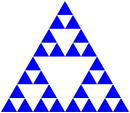
And each of those.
And so on.
And so forth.
If we do this process sufficiently many times (perhaps "arbitrarily many times"), we end up with a structure called the "Sierpinski Triangle". Sierpinski triangles have many surprising mathematical properties, none of which are relevant to us at this time. Instead, we will use Sierpinski triangles to make cool-looking drawings!
We will start by defining the intermediate results recursively.
Here's one way.
We'll call a triangle that's been broken up n times a "level-n fractal triangle".
- A level-0 fractal equilateral triangle with edge-length
lenis just an equilateral triangle of edge-lengthlen. - A level-n fractal equilateral triangle with edge-length
lenis built from three level-(n-1) fractal equilateral triangles, each with edge-lengthlen/2. For example, a level-5 fractal equilateral triangle with side-length 128 is built from three level-4 equilateral triangles, each with side length 64.
You can turn that into a recursive procedure, can't you? Don't worry; you'll have a chance to do so in the exercises below.
Once we can build fractal triangles, we can start varying them. For example, rather than making each sub-triangle the same color, we might make one lighter and another darker. If we use the "standard" technique of adding 32 to each color component to make colors "lighter" and subtracting 32 to make them "darker", we might end up with something like the following for a level-4 gray triangle.
Here's another one that we've built by making the top triangle redder, the bottom-left triangle greener, and the bottom-right triangle bluer. (I think this has six levels of recursion.)
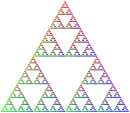
And one where we've turned each middle triangle into the base color. (We've done that by overlaying the recursive result on a larger triangle.)
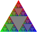
It looks a bit different if we just overlay the first one on gray.
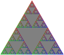
When we do enough recursion, it may not matter all that much whether or not the base case is a triangle. (Is that surprising or intuitive?) For example, here are a set of shapes using the (above shape (beside shape shape)) formula with a square as the base case.

Somewhere along the way, I think we said that these techniques might help us make compelling (or repelling?) images. Here's an experiment with using that last approach with seven shades of red and then overlaying them.
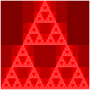
Required "tests" for drawing functions
In this assignment, we don't have a good way to test your code for correctness automatically! The starter code provides example invocations of your functions that you should check. However, in addition to these examples, you should provide two additional invocations of each function, demonstrating different behavior than what the given examples show. When writing these examples:
- Write your two additional examples below the given examples in the appropriate section.
- Give each example an appropriate description with the
descriptionfunction. - Please ensure that your code runs to completion in a reasonable amount of time! In other words, don't give your examples inputs that will take the program longer than a few seconds to execute!
Part one: Fractal triangles
Problem 1a: fractal-triangle
Write a procedure, fractal-triangle, that makes the basic fractal triangle described above.
;;; (fractal-triangle side color n) -> image?
;;; side : positive-real?
;;; color : rgb?
;;; n : non-negative integer
;;; Make a fractal triangle of the given side length using `color` as
;;; the primary color.
Warning: Because shapes generally can't have fractional width or height, you may find that fractal-triangle produces triangles that are slightly bigger than expected. Such a result is acceptable. You'll notice all of our tests use a size that's a power of two to address such issues.
Problem 1b: rgb-fractal-triangle
Write a procedure, rgb-fractal-triangle, that makes a fractal triangle in which the top triangle is "redder" than the basic color, the lower-left triangle is "greener" than the basic color, and the lower-right triangle is "bluer" than the basic color.
;;; (rgb-fractal-triangle side color n) -> image?
;;; side : positive-real?
;;; color : rgb?
;;; n : non-negative integer
;;; Make a fractal equilateral triangle of the given side length using
;;; `color` as the primary color. In the recursive steps, the base
;;; color of the top triangle is `(rgb-redder color)`, the base color
;;; of the lower-left triangle is `(rgb-greener color)`, and the base
;;; color of the lower-right triangle is `(rgb-bluer color)`.
Problem 1c: new-rgb-fractal-triangle
As you saw in our examples, once we start changing colors, it can be nice to "fill in" the center triangle with the original color. You will find it easiest to do so by overlaying the fractal triangle on a same-size triangle in the original color.
Write a procedure, (new-rgb-fractal-triangle side color n), that does just that.
;;; (new-rgb-fractal-triangle side color n) -> image?
;;; side : positive-real?
;;; color : rgb?
;;; n : non-negative integer
;;; Make a fractal equilateral triangle of the given side length using
;;; `color` as the primary color. In the recursive steps, the base
;;; color of the top triangle is `(rgb-redder color)`, the base color
;;; of the lower-left triangle is `(rgb-greener color)`, and the base
;;; color of the lower-right triangle is `(rgb-bluer color)`. The base
;;; color of the central triangle should be `color`.
Problem 1d: fractal-right-triangle
Write a procedure, (fractal-right-triangle width height color n), that builds a right triangle using the fractal approach.
;;; (fractal-right-triangle height width color n) -> image?
;;; width : positive-real?
;;; height : positive-real?
;;; color : color?
;;; n : non-negative integer
;;; Make a fractal right triangle using `color` as the primary color.
Part two: Fractal squares (carpets)
Just as we can think of triangles as being made up of four sub-triangles, and we can use that idea to make fractal triangles, we can break squares up into sub-squares and use those to make fractal squares.
The most common approach is to make a three-by-three grid of squares, building all but the center square recursively.
How do we combine them?
We can make each row with beside and then stack the three rows with above.
What about the middle square, which we normally leave "blank"?
I find it easiest to specify a color to use for the center.
Here are the first few stages.

No, the limit of this is not a "Sierpinski square". However, it is normally referred to as a Sierpinski carpet".
Problem 2a. carpet-a
Write a procedure, (carpet-a size color-x color-y n) that makes an image like those above.
;;; (carpet-a size color-x color-y n) -> image?
;;; size : positive real?
;;; color-x : color?
;;; color-y : color?
;;; n : non-negative integere
;;; Create a `size`-by-`size` image of the standard fractal carpet with
;;; `n` levels of recursion, using `color-x` as the "primary" color and
;;; `color-y` as the center color.
Problem 2b. carpet-b
Of course, there's no reason we have to recurse on those particular eight squares. We could, for example, use only six. Here's one such pattern.

Here(and elsewhere, we are seeing some strange artifacts from our squares having non-integer edge lengths.)
Write a procedure, (carpet-b size color-x color-y n), that makes images like this latest set.
;;; (carpet-b size color-x color-y n) -> image?
;;; size : positive real?
;;; color-x : color?
;;; color-y : color?
;;; n : non-negative integer.
;;; Create a `size`-by-`size` image of a fractal carpet with `n` levels
;;; of recursion, using `color-x` as the "primary" color and `color-y`
;;; as the "secondary" color. Our pattern looks something like this.
;;;
;;; X y X
;;; y y X
;;; X X X
;;;
;;; where `X` means "recurse" and `y` means "square with `color-y`.
Problem 2c: carpet-c
Those big squares really stand out, don't they?
But we can handle that.
Instead of just making a rectangle of color-y, we can recurse in those squares, too, flipping the primary and secondary colors.
Here are the first few versions with that model, using the same pattern as in carpet-b.

Write a procedure, (carpet-c size color-x color-y n), that makes images like the latest set.
;;; (carpet-c size color-x color-y n) -> image?
;;; size : positive real?
;;; color-x : color?
;;; color-y : color?
;;; n : non-negative integer.
;;; Create a `size`-by-`size` image of a fractal carpet with `n` levels
;;; of recursion, using `color-x` as the "primary" color and `color-y`
;;; as the "secondary" color. Our pattern looks something like this.
;;;
;;; X Y X
;;; Y Y X
;;; X X X
;;;
;;; where `X` means "recurse keeping colors as they are" and `Y` means
;;; "recurse swapping the two colors".
Problem 2d: carpet-d
d. Just as we can recurse on the secondary squares, we can choose not to recurse on some of the primary color squares. Here's an example with a somewhat different pattern. You can see if you can determine the pattern by inspection, or you can read the documentation.

Write a procedure, (carpet-d size color-x color-y n), that makes images like the latest set.
;;; (carpet-d size color-x color-y n) -> image?
;;; size : positive real?
;;; color-x : color?
;;; color-y : color?
;;; n : non-negative integer.
;;; Create a `size`-by-`size` image of a fractal carpet with `n` levels
;;; of recursion, using `color-x` as the "primary" color and `color-y`
;;; as the "secondary" color. Our pattern looks something like this.
;;;
;;; X y X
;;; x Y x
;;; X y X
;;;
;;; where `X` means "recurse keeping colors as they are", `Y` means
;;; "recurse swapping the two colors", `x` means "square in `color-x`"
;;; and `y` means "square in `color-y`".
Problem 2e: carpet
At this point, you may feel like you want to experiment with different patterns of carpet recursion.
And you could do so by making slight changes to carpet-d.
However, it's much better to extend our procedure to take the pattern of recursion as a parameter.
For example, the "pattern" for carpet-d is "XyXxYxXyX".
Write a procedure, (carpet pattern size color-x color-y n), that generalizes carpet generation using patterns.
(Note: This procedure is only required for an E.)
;;; (carpet pattern size color-x color-y n) -> image?
;;; pattern ; string? (length 9, composed only of x, X, y, and Y)
;;; size : positive real?
;;; color-x : color?
;;; color-y : color?
;;; n : non-negative integer.
;;; Create a `size`-by-`size` image of a fractal carpet with `n` levels
;;; of recursion, using `color-x` as the "primary" color and `color-y`
;;; as the "secondary" color.
;;;
;;; The pattern is given by the letters in pattern, where `X` means
;;; "recurse" keeping colors as they are", `Y` means "recurse swapping
;;; the two colors", `x` means "square in `color-x`" and `y` means
;;; "square in `color-y`".
;;;
;;; The positions of the letters correspond to the parts of the pattern
;;;
;;; 0 1 2
;;; 3 4 5
;;; 6 7 8
Part three: Freestyle
Using variants of the fractal approaches from parts 1 and 2, along with anything else you consider useful, come up with a recursive procedure, (my-fractal size color n) that creates a self-similar (or otherwise numerically recursive) image using the starting size, color, and non-negative integer.
Include three invocations of my-fractal that demonstrate your fractal on a variety of inputs.
Grading rubric
Redo or above
Submissions that lack any of these characteristics will get an N.
- Displays a good faith attempt to complete every required part of the assignment.
Meets expectations or above
Submissions that lack any of these characteristics but have all the prior characteristics will get an R.
- Includes the specified file,
fractals.scm. - Includes an appropriate header on all submitted files that includes the course, author, etc.
- Correctness
- Code runs without errors.
- Core functions are present and correct (except for non-obvious corner cases, when present)
- Part 1:
(fractal-triangle side color n)(rgb-fractal-triangle side color n)(new-rgb-fractal-triangle side color n)(fractal-right-triangle width height n)
- Part 2:
(carpet-a size color-x color-y n)(carpet-b size color-x color-y n)(carpet-c size color-x color-y n)(carpet-d size color-x color-y n)
- Part 1:
- Each function has two additional invocations beyond what is provided in the starter code.
- Design
- Documents and names all core procedures correctly.
- Code generally follows style guidelines.
my-fractalinvolves explicit or implicit recursion other than from invoking procedures in parts 1–3.
Exemplary / Exceeds expectations
Submissions that lack any of these characteristics but have all the prior characteristics will get an M.
- Correctness
- Implementation of all core functions is completely correct, even in non-obvious corner cases when present.
- Each set of tests includes at least one edge case (e.g., an empty list, if appropriate).
- Extra functions are present and completely correct:
- Part 2, problem 2e:
(carpet pattern size color-x color-y n)
- Part 2, problem 2e:
- Design
- Function documentation is complete and appropriately evocative of each function's behavior.
- Code follows style guidelines completely, with at most three minor errors present.
- Code is well-designed, avoiding repeated work through decomposition and appropriate language constructs.
my-fractalinvolves a basic shape other than triangles, squares, and rectangles.
Recursion over Numbers
The heart of our recursive functions so far is our recursive definition of lists:
A list is either:
- Empty (
null) or- Non-empty (
(cons head tail)) with aheadelement and a sub-list, itstail.
Our recursive functions mirror this recursive definition. So it stands to reason that if we are able to give a recursive definition for any type, then we can perform recursion over that type similarly!
Many kinds of data admit recursive definitions, and you will encounter many of them throughout your computer science journey. However, there is one datatype that trumps them all---perhaps even more so than a list! It is the natural number. Recall that the natural numbers are the non-negative integers. This includes the numbers , , , , ..., etc.
Our definition of a list was recursive because at least one of the cases included a smaller list inside itself.
head [ tail ]
^ ^
| |
element sublist
We can see via the picture where the smaller list is located: it's the tail of the list! However, now let's consider a natural number, say :
5
Ugh. Unlike lists, it is not immediately obvious what the "smaller" natural number is in this situation. Where is it hiding?
One way to discover where the smaller natural number exists inside of is to answer the following question: how can we express in terms of some small natural number? This perspective opens up many possibilities! For example, the following expressions all evaluate to :
- .
- .
- .
And so forth. Of these options, addition-by-one is most like the head-tail relationship for lists. Let's compare the two perspectives:
- Consider the list
(list 1 2 3 4 5). We can express this list as(cons 1 (list 2 3 4 5))where1is the head and(list 2 3 4 5)is the tail. We join the head and tail to form the overall list withcons. - Consider the natural number .
We can express this natural number as
(+ 1 4)where is the smaller natural number. We add one to this number to obtain the natural number .
In general, we call the successor of the smaller natural number . We can see that almost every natural number has a successor:
- is the successor of .
- is the successor of .
- is the successor of .
However, because natural numbers are non-negative integers, is not a successor of any other number. It is the base case for our recursive natural number definition! Combining these two ideas, we arrive at our recursive definition for the natural numbers:
A natural number is either:
- Zero or
- The successor or "plus one" of a smaller natural number.
With this definition, we can solve problems using recursive decomposition on natural numbers!
Example: Factorial
A classical example of a mathematical function with a recursive definition is factorial, written . is the product of the numbers from to , e.g., . In general, .
Suppose we were to go to implement a factorial function that returns when given an natural number argument n.
We can't implement the "⋯" in Scheme directly, so we need to find some alternative way of expressing this computation.
Let's see if we can find a recursive decomposition for factorial in terms of our recursive definition for the natural numbers:
To compute the factorial of some natural number
n:
- When
nis zero... (a)- When
nis non-zero... (b)
-
When
nis zero, we should return0!. But what is0!? It turns out that the factorial function is defined so that is 1. This seems arbitrary since asking the question "multiply the numbers from 1 to 0" is a malformed question! Indeed, we define by convention because it makes our mathematical formulae work without the need for special cases. -
When
nis non-zero, it is the successor of some smaller number, call itkwith . How can I express factorial of in terms of factorial of ? Let's look at a concrete example: suppose so . We have:In terms of recursive design, our recursive assumption says we can compute . How can we then compute in terms of ? We can see above that . We can then generalize this idea to conclude that when is non-zero, .
This gives us a final recursive decomposition for factorial:
To compute the factorial of some natural number
n:
- When
nis zero, the factorial of0is1by definition.- When
nis non-zero, the factorial ofnis the factorial ofn-1timesn.
We can then translate this decomposition directly into our desired function:
(import test)
(define factorial
(lambda (n)
(if (zero? n)
1
(* n (factorial (- n 1))))))
(test-case "factorial zero"
= 1
(lambda ()
(factorial 0)))
(test-case "factorial non-zero"
= 120
(lambda ()
(factorial 5)))
Note that we use the zero? function to test whether n is zero which works only because we assume as a precondition that n is a natural number, i.e., non-negative.
We could also instead choose to use a comparison operator, e.g., (= n 0) or (> n 0) (and flip the order of the conditional branches), to achieve the same effect.
To access the predecessor of n (i.e., the number of which n is a successor), we use subtraction.
Alternatively, we can also use pattern matching, passing in an appropriate numeric literal for the base case:
(import test)
(define factorial
(lambda (n)
(match n
[0 1]
[_ (* n (factorial (- n 1)))])))
(test-case "factorial zero"
= 1
(lambda ()
(factorial 0)))
(test-case "factorial non-zero"
= 120
(lambda ()
(factorial 5)))
In the recursive case, we can't use a pattern to bind the number "one less than n."
So instead, we use a wildcard pattern, _ to match anything that reaches the second branch.
Note that match expressions are consumed in top-down order, so if n is not 0, then---assuming n is a natural number---it is non-zero, so the second branch should always apply.
For numeric recursion, i.e., recursion over the natural numbers, you should feel free to use either pattern matching or an appropriate if or cond expression.
One final thing to observe is that the standard recursive definition of factorial typically presented as:
Aligns very closely with the pattern matching version of our code. Indeed, pattern matching in programming comes from the use of pattern matching to elegantly define functions in mathematics. Because programming draws on mathematics so much, we typically find that pattern matching allows us to concisely describe mathematical algorithms.
Applying Numeric Recursion
We can use numeric recursion to implement recursively defined mathematical functions. However, what elevates numeric recursion to such importance is that we can express many recursive patterns in terms of the natural numbers! Indeed, the natural numbers form an ordering:
So we expect that if a data structure or algorithm can be expressed in some "ordered" fashion, we can use numeric recursion! For example, consider the recursively defined triangles that motivated our initial exploration into recursion:
(import image) (overlay (triangle 250 "outline" "blue") (triangle 225 "outline" "blue") (triangle 200 "outline" "blue") (triangle 175 "outline" "blue") (triangle 150 "outline" "blue") (triangle 125 "outline" "blue") (triangle 100 "outline" "blue") (triangle 75 "outline" "blue") (triangle 50 "outline" "blue") (triangle 25 "outline" "blue"))
This code is clearly redundant! How can we use numeric recursion to capture the recursive nature of this pattern?
To do so, we can observe that there is are two potential "order" to the triangles: we can think about drawing them from top-to-bottom according to our overlay invocation or in the other order, from bottom-to-top.
Let's generalize this computation to draw an arbitrary number of triangles, so let's draw them bottom-to-top, i.e., inside out, so that we can draw an unbounded number of triangles!
Our recursive decomposition will decompose the task of drawing n such triangles:
To draw
ntriangles:
- When
nis zero... (a)- When
nis non-zero... (b)
-
When is zero, we should draw no triangles! But how can we create a drawing that contains no triangles? One way out of this conundrum is to simply draw a triangle of size which will not appear on the screen.
-
When is non-zero, we need to draw triangles by first recursively drawing triangles---that's our recursive assumption. How do we then draw the th additional triangle? We need a formula for the size of the th triangle in terms of ! To derive this, let's put the sizes in a table according to their order according to the natural numbers. Alternatively, we can think of the number as their index in the ordering:
- , .
- , .
- , .
- , .
- , .
By observing the pattern and using algebra, we can see that the size of triangle is . We can then use
overlayto combine the th triangle with the remaining triangles.
This gives us our final decomposition:
To draw
ntriangles:
- When
nis zero, draw a triangle with size .- When
nis non-zero, overlay a triangle of size with a drawing of triangles.
Again, we can translate this decomposition into code directly:
(import image)
(define nested-triangles
(lambda (n)
(match n
[0 (triangle 0 "outline" "blue")]
[_ (overlay (triangle (* n 25) "outline" "blue")
(nested-triangles (- n 1)))])))
(nested-triangles 10)
(nested-triangles 5)
(nested-triangles 0)
(nested-triangles 25)
Self-checks
Problem: The Termial
If factorial is the operation that performs repeated multiplication, then we call the operation that performs repeated addition the terminal. For example:
(terminal 10)
> 55
(terminal 0)
> 0
- Follow the example of
factorialand give a recursive decomposition forterminal. - Implement the
terminalfunction based on this decomposition.
Problem: By Size (‡)
We defined (nested-triangle n) to draw n triangles.
Effectively, each triangle drawn by the function decreased in size by 25 which we derived in our recursive decomposition.
Instead of drawing n triangles, we can instead take the size of the largest triangle as input and decrease that size by 25 directly, instead of computing it as a formula of the number of triangles n.
- Give a recursive decomposition for an alternative implementation of
(nested-triangle size)that takes the size of the overall image as input. Thesizehere becomes thesizeof the outermost triangle, and each successive triangle decreases by25down to0. For example(nested-triangle 250)should produce our original example of10triangles. - Implement this alternative decomposition of
(nested-triangle size)and figure out whichsizeparameters produce the examples generated in the reading. - Think about the pros and cons of this new implementation of
nested-triangle. Is there any upsides or downsides to having the parameter of the function be the size of the drawing versus the number of triangles?
Numeric recursion
In this lab, we'll continue our exploration of recursion by considering how we might recurse over numbers.
Preparation
- Introduce yourself to your partner, discuss strengths and weaknesses, agree upon work procedures, etc.
- The person nearest the board is Side A. The other person is Side B. Grab the code from
- Review the procedures included in the lab to make sure you understand what they are intended to do.
Implementing the Big Three
In this lab, we'll combine higher-order functions and recursion to see how to implement map, filter, and fold.
Preparation
- Introduce yourself to your partner, discuss strengths and weaknesses, agree upon work procedures, etc.
- The person nearest the board is Side A. The other person is Side B. Grab the code from:
Tail Recursion
So far, we have not dwelled too much on program efficiency. By program efficiency, we mean two qualities:
- Time efficiency: how long a program takes to run?
- Space efficiency: how much memory does a program consume during execution?
We will cover efficiency in depth in later courses. However, today we'll cover a particular problem of efficiency as it pertains to recursion and functional programming. Our solution to this problem, tail recursion, is a fundamental part of every functional programming language.
Blowing the Stack
Consider the function (make-list n v) which makes a list of n copies of v, implemented recursively:
(define make-list
(lambda (n v)
(if (= n 0)
null
(cons v (make-list (- n 1) v)))))
And let's trace its execution on an example:
(make-list 5 "z")
-->* (cons "z" (make-list 4 "z"))
-->* (cons "z" (cons "z" (make-list 3 "z")))
-->* (cons "z" (cons "z" (cons "z" (make-list 2 "z"))))
-->* (cons "z" (cons "z" (cons "z" (cons "z" (make-list 1 "z")))))
-->* (cons "z" (cons "z" (cons "z" (cons "z" (cons "z" (make-list 0 "z"))))))
-->* (cons "z" (cons "z" (cons "z" (cons "z" (cons "z" null)))))
-->* (list "z" "z" "z" "z" "z")
Observe the "essence" of this computation: for every element of the input list, we "pop out" a (cons "z" ...) call.
These cons calls do not immediately evaluate!
Instead, we continue making recursive calls until we hit the base case.
It isn't until after this point that we evaluate the five cons calls that we accumulate along the way.
Looking at the trace, we see that if we pass in n to make-list, after k calls of make-list, we will have n-k pending calls to cons built up as we continue with the recursion:
(cons "z" (cons "z" (cons "z" ... (cons "z" (make-list (- n k) "z")))))
\ /
-----------------------------------------
|
k
Observe that our mental model of computation suggests that our computer must store these pending calls somewhere!
Each (cons "z" ...) call represents the work that a particular call to make-list must do after it makes its recursive call.
Indeed, behind the scenes, our program maintains a call stack, the collection of currently active function calls that are waiting to complete.
The call stack contains a stack frame for each active function call that records the information necessary for that function to continue when any function calls it makes finishes execution.
For five elements, this additional work does not seem to be a problem, but imagine if we tried to call make-list with, say, n = 1000000.
We would need to allocate a million stack frames to perform this computation!
To put this into context, let's imagine that a single stack frame, for simplicity's sake, is only 4 bytes big, an underestimate.
(A byte, or 8 bits, is an elementary unit of data in a computer system.)
We would need to allocate or 4 megabytes (MB) of stack frames.
It turns out that most programming language runtimes only allow for stacks to grow to, at most, several megabytes, so that the system's memory can be used for other tasks.
When we run out of stack space to record active function calls, our programs raise a stack overflow error indicating that it has run out of memory! These physical limits of memory become a problem in functional programming because we use recursion to perform our repetitive tasks. While we haven't encountered this problem yet, real-world programs might process data that contains millions or even billions of elements. Naively performing recursive computation in these situations simply does not work!
(As an aside, stack overflow errors are precisely why we haven't seen "true" infinite loops in our programs. In virtually all of the recursive functions we've written so far, we would overflow the stack with an infinite loop, causing an error!)
Tail Recursion
Consider this alternative version of make-list:
(define make-list
(lambda (so-far n v)
(if (= n 0)
so-far
(make-list (cons v so-far) (- n 1) v))))
This version of make-list takes an extra argument, so-far, that represents the result of the function accumulated so far in its execution.
Let's trace execution of this function on the same example.
Note that we pass so-far the initial value of null capturing the fact that, initially, we have not yet done any computation.
(make-list null 5 "z")
-->* (make-list (cons "z" null) (- 5 1) "z")
-->* (make-list (list "z") 4 "z")
-->* (make-list (cons (list "z")) (- 4 1) "z")
-->* (make-list (list "z" "z") 3 "z")
-->* (make-list (cons "z" (list "z" "z")) (- 3 1) "z")
-->* (make-list (list "z" "z" "z") 2 "z")
-->* (make-list (cons "z" (list "z" "z" "z")) (- 2 1) "z")
-->* (make-list (list "z" "z" "z" "z") 1 "z")
-->* (make-list (cons "z" (list "z" "z" "z" "z")) (- 1 1) "z")
-->* (make-list (list "z" "z" "z" "z" "z") 0 "z")
-->* (list "z" "z" "z" "z" "z")
Observe how the "computation" occurs on the so-far argument rather than the result of the recursive call.
We incrementally cons on an additional "z" onto so-far for each recursive call to the function.
This cons is resolved before the next call to make-list is made.
Critically, because we evaluate arguments before calling functions, each recursive call of make-list perform its computation before it makes its recursive call.
As evidenced by our derivation, there is no work to do after the recursive call.
Such a pattern of recursion is called tail recursion and a function that exhibits this behavior is said to be in tail-recursive form.
Definition (Tail-Recursive Form): a function is in tail-recursive form if, for every recursive function call that it makes, that no additional work is performed after that call. In other words, a tail recursive function immediately returns the result of any recursive call that it makes.
The second version of make-list is in tail-recursive form because it simply returns the result of its recursive call in its else-branch.
In contrast, the first make-list is not in tail-recursive form because it performs a (cons ...) call after it makes its recursive call.
Importantly, when a recursive function is in tail-recursive form, our language can perform an important optimization called tail-call optimization.
If we look at our trace of the second make-list call, we see that our executing program never "grows" like the first case.
Behind the scenes, this means that we do not need to keep around each stack frame for a tail-recursive call because we perform no work after that call is made---we simply return whatever the recursive call returns.
This is strictly more efficient in terms of memory usage than regular recursive calls!
Tail-call optimization is so important in functional programming that most functional programming languages mandate that their interpreters and compilers must perform tail-call optimization so that programs can perform unbounded recursion, provided that functions are written in tail-call style. Scamper does not yet support tail-call optimization---it turns out to be quite a non-trivial program transformation behind the scenes. But this pattern is prevalent enough in real-world functional programming that it is important to internalize, even without the benefits!
Converting Functions to Tail-recursive Form
We can see that make-list can be rewritten in tail recursive form.
What about other recursive functions?
Let's revisit the list length function:
(define length
(lambda (l)
(match l
[null 0]
[(cons _ tail) (+ 1 (length l))])))
length is not in tail-recursive form because it performs additional computation after its recursive call, (+ 1 ...).
Our goal in converting functions to tail-recursive form is to ensure that the function immediately returns the result of any recursive calls that it makes.
Or to put it another way, we need to rewrite length so that it performs no additional computation after its recursive calls.
The key to this transformation is transferring any work done after a recursive call to before the recursive call, usually by performing that computation as an argument to the function.
Such a transformation is impossible without modifying the signature of length.
In particular, we'll add an argument, conventionally named so-far, to perform this computation over.
Observe how the (+ 1 ...) performed on the recursive call is moved to the so-far argument.
Additionally, we modify the base case to return so-far.
When we hit the base case, we're done with the computation
If so-far is the work performed so far in the recursive computation, so-far should contain the completed computation at the base case, so we return it directly.
Finally, we create a wrapper function that calls our recursive function, but with an appropriate initial argument for so-far.
This wrapper function becomes the length function that users call, and we call the recursive function the helper function that does the actual work.
The initial value for so-far is the value returned by the base case in the original version of the function.
(import test)
(define length-helper
(lambda (so-far l)
(match l
[null so-far]
[(cons _ tail) (length-helper (+ 1 so-far) tail)])))
(define list-length
(lambda (l)
(length-helper 0 l)))
(test-case "list-length: non-empty"
equal? 5
(lambda ()
(list-length (list 1 2 3 4 5))))
It is instructive to state the recursive decomposition of length-helper and compare it to our decomposition of length:
-
lengthThe length of a list
l:- If
lis empty, then the length oflis zero. - If
lis non-empty, then the length oflis one plus the length of its tail.
- If
-
length-helperThe length of a list
l, provided we computed the lengthso-far:- If
lis empty, then the length is the length we computedso-far. - If
lis non-empty, then the length is the length of the tail, observing we have computed one plusso-farfor the length.
- If
When decomposing a problem recursively in a tail-call style, we define the computation in terms of what has been computed "so far."
Generalizing Tail-call Conversion
While it is not obvious, it turns out that we can convert any recursive function into tail-recursive form by following the pattern we outlined above:
- Create a recursive helper function that does the actual work of the function.
This function should take an additional argument,
so-far, that records the results of the computation before recursive calls are made. - Define the recursive helper function similarly to the original function, except:
- The base case should return
so-farsinceso-farshould contain the overall result at this point in the computation. - The recursive case should have any work it does after its recursive calls moved to the
so-farargument passed to those recursive calls.
- The base case should return
- Create a wrapper function with the desired function's signature that simply calls the helper with a suitable initial value for the
so-farargument.
In our examples, so-far has been a simple value that we've updated.
More generally, we can expect so-far to become a function that represents the accumulated work to be done so far.
In this formulation, so-far is called a continuation and the transformation is called continuation-passing style (CPS) where every function accept its continuation, i.e., what to do after the function completes execution.
While seemingly weird and unnatural, it turns out continuation-passing style is useful in many contexts, even outside functional programming.
For example, CPS is employed as a pattern in the Javascript programming language for writing asynchronous, callback-based code.
Self Checks
Exercise 1: Tracing Tail-recursive Functions
Use your mental model of evaluation to give a step-by-step trace of (length (list 1 2 3 4 5)) for both the non-tail-recursive and tail-recursive versions of length, demonstrating that the former implementation requires work done after each recursive call and the latter does not.
Exercise 2: Tail-recursive Decompositions
Give prose-based recursive decompositions for the original make-list function and its tail-recursive variant.
Exercise 3: Tail-recursive Append (‡)
Translate the standard implementation of append into tail-recursive form:
(import test)
(define list-append
(lambda (l1 l2)
(match l1
[null l2]
[(cons head tail) (cons head (list-append tail l2))])))
(test-case "list-append: non-empty"
equal? (list 1 2 3 4 5)
(lambda ()
(list-append (list 1 2 3)
(list 4 5))))
Tail and helper recursion
In this lab, we'll further expand our understanding of recursion, considering how patterns (both pattern matching and patterns of recursion) and helper procedures improve our ability to recurse.
Preparation
- Introduce yourself to your partner, discuss strengths and weaknesses, work procedures, and such.
- Go over your answers to the self checks.
- Grab the code.
- Review the provided procedures.
Acknowledgements
This lab was rewritten in Spring 2023 based on previous tail recursion labs, the most recent of which was Fall 2021.
Association Lists
In this course, we explore two broad classes of data structures:
- Sequences that associate elements in a sequential fashion. We represent sequences in Scheme primarily with lists.
- Hierarchies that establishes parent-child relationships between elements. We represent hierarchies in Scheme primarily with trees (which we will discuss in the last third of the course).
However, are there any other kinds of relationships we might establish between data? If such relationships exist, how do we capture them in Scheme?
As a motivating example, consider writing a program that captures the inventory of an online store. In particular, we have identified that for each item the store sells, we need to record how many of that item we have in the warehouse. We also expect to perform three operations on our inventory:
- Given an item, determine if our inventory has an entry for that item.
- Given an item, lookup the amount of that item we have in the inventory.
- Given an item and a new amount, update the inventory entry for that item with the given amount.
For example, we might note in our inventory we have:
"apples" -> 5
"bananas" -> 2
"oranges" -> 8
Here are some sample outcomes of our operations over this example inventory:
- The inventory has an entry for
"apples". The inventory does not have an entry for"grapes". - The inventory has an entry mapping
"bananas"onto2, i.e., the inventory has two bananas. Likewise, the inventory records that we have eight oranges. - If someone buys two applies, we can update the inventory by first looking up the number of apples originally in the inventory, subtracting two from that amount, and then updating the entry for apples with the new amount,
5 - 2 = 3.
In all of these cases, we operate over a collection of mappings. The mappings in question are the three inventory entries above, which associates fruits to numbers. Note that the mappings are ultimately arbitrary: any fruit can be assigned any (non-negative) integer value.
In computer science, the class of data structures that captures these sorts of arbitrary mappings between elements is called a map or a dictionary. The name "dictionary" is evocative of the prototypical example of these kinds of data structures: a mapping from a word to its definition. We say that the keys of the dictionary are the values we're "mapping from"—fruits in our example. The values of the dictionary are the values we're "mapping to"—numbers in our example.
An Aside: Pairs in Scheme
In our dictionary data structure, we will need to associate a key with a value.
The simplest way of doing this is with a pair structure which holds two values.
For example, we can represent - coordinates in a two-dimensional space by using the pair function to create a pair.
To get out the components of a pair we use the car and cdr functions:
(define origin (pair 0 0))
(display (pair 0 0))
(define translate
(lambda (p dx dy)
(pair (+ (car p) dx) (+ (cdr p) dy))))
(display (translate origin 3 5))
But wait, we used car and cdr to access the head and tail of lists!
(define lst (range 0 10)) (display (car lst)) (display (cdr lst))
How can car and cdr serve these two different roles?
The answer is both surprisingly simple but also thought-provoking: a list is a pair!
More specifically a list is a pair of a value and a list, recursively!
So null is a list, a pair of a value and null is a list, a pair of a value and a pair of a value and null is a list, and so forth!
(display null)
(display
(pair 5 null))
(display
(pair "a"
(pair 5 null)))
If the last component is not a list, Scamper will happily display the value as the collection of nested pairs that the value really is:
; Observe how the nested pairs "bottom out" to
; a number instead of a list.
(display
(pair "a"
(pair 5 0)))
In this sense, you can think of a value being displayed as a list as convenient short-hand for nested pairs that meet this criteria!
Dually, as you see above, cons and pair are interchangable—both produce pairs that may or may not be considered lists!
A final note here is that because pairs and lists are interchangable, we can also use pattern matching to concisely access both elements of a pair.
Here is the redefinition of the translate function above but using pattern matching.
Note that the elementary pair value is cons rather than pair, so we need to pattern match on the cons constructor:
(define origin (pair 0 0))
(define translate
(lambda (p dx dy)
(match p
[(cons x y) (pair (+ x dx) (+ y dy))])))
(display (translate origin 3 5))
Association Lists
With this in mind, how might we implement a dictionary? We can implement dictionaries by using a combination of lists and pairs, creating a structure called an association list.
-
Individual mappings between elements can be captured with pairs. For example
(pair "apples" 5)can represent the association of the string"apples"to the number5. -
Collections of these mapping can be gathered up in a list, e.g., our complete inventory can be represented by the following list of pairs:
(list (pair "apples" 5) (pair "bananas" 2) (pair "oranges" 8))
With an implementation in mind, we can now talk about how we might implement the major operations over dictionaries we described above:
(assoc-key? k lst): returns true if association listlstcontains an entry keyk.(assoc-ref k lst): returns the value associated with keykin association listlst.(assoc-set k v lst): returns a association list that islstwith an updated entry associating keykwith valuev.
On top of this, we also note that the empty association list is simply the empty list, i.e.,
;;; The empty association list (contains no entries) (define assoc-empty null)
Since we know that the implementation of our dictionary is a list of pairs, we can write recursive implementations of each of these functions, and we'll do so in lab as an exercise.
For example, assoc-key? is realized by the following recursive decomposition over the input list l:
Association list
lcontains keykas follows:
- When
lis empty, there are no entries, soldoes not containk.- When
lis non-empty, let the head oflbe somekeyandvaluepair. Ifkis equal tokey, thenlcontainsk. Otherwise,lcontainskonly if the tail oflcontainsk.
The following implementation realizes this decomposition:
(import test)
(define my-assoc-key?
(lambda (k l)
(match l
[null #f]
[(cons (pair key _) tail) (if (equal? k key) #t (my-assoc-key? k tail))])))
(define example (list (pair 0 "foo") (pair 1 "bar") (pair 2 "baz")))
(test-case "my-assoc-key? empty"
equal?
#f
(lambda () (my-assoc-key? 0 null)))
(test-case "my-assoc-key? non-empty in"
equal?
#t
(lambda () (my-assoc-key? 1 example)))
(test-case "my-assoc-key? non-empty not in"
equal?
#f
(lambda () (my-assoc-key? 42 example)))
Note that Scheme provides implementations of these functions in the standard library! Here is an example program that shows how we can fully realize our example fruit inventory in Scheme, complete with the operations from the standard library:
(define inventory (list (pair "apples" 5) (pair "bananas" 2) (pair "oranges" 8))) (display inventory) (assoc-key? "apples" inventory) (assoc-key? "grapes" inventory) (assoc-ref "apples" inventory) (assoc-ref "bananas" inventory) (assoc-ref "oranges" inventory) (define updated-inventory (assoc-set "apples" 3 inventory)) (display updated-inventory) (assoc-ref "apples" updated-inventory) (assoc-ref "bananas" updated-inventory) (assoc-ref "oranges" updated-inventory)
Self-Check (‡)
Note that assoc-set replaces or overwrites an entry for a given key by appending to the front of the association list.
Frequently we want to update that entry instead.
That is, given the old value in the entry, update the entry in terms of some updating value.
Let's consider a specialized version of this update functionality in terms of our inventory.
Write a function (assoc-update-inc-by d k n) that returns a new dictionary that is d but updates key-value pair (pair k v) of d to be (k (+ v n)).
That is, we add n to the value associated with k in d.
We could apply the function to concisely write the behavior described in our example as follows:
> (assoc-update-inc-by inventory "apples" -2)
(list (cons "apples" 3) (cons "bananas" 2) (cons "oranges" 8))
(Hint: follow the pattern for assoc-key? but instead of merely returning a boolean, return a new pair containing the desired update!)
Letter Inventory
In this laboratory, we'll explore the association list data structure and a novel application of the data structure: frequency analysis of letters in text.
- Introduce yourself to our partner and discuss work procedures.
- Decide whom is partner A and partner B for the purposes of pair programming for this lab.
- Complete the definitions in the file below and turn it into Gradescope when you are done:
Take-home assessment 7: musical improviser
Musical improvisation is the act of creating and performing a musical composition "on the spot." A hallmark of many modern musical genres such as rock, blues, and jazz, improvisation requires both technical mastery and creativity of the musician. In this assessment, you will build a simple improviser using randomness. We'll then observe that we this simple improviser doesn't sound so great!
Logistics and turn-in
You should write your program in a file called improv.scm and use the lab library to structure your program according to the parts outlined in this write-up:
;;; improv.scm ;;; A musical improviser ;;; CSC-151-XX 24fa. ;;; ;;; Author: Your Name Here ;;; Date submitted: YYYY-MM-DD ;;; ;;; Acknowledgements: ;;; ;;; * ... ;;; * ... (import lab) (title "A musical improviser") (part "Part 1: Infrastructure) (part "Part 2: A basic improviser") (part "Part 3: Licks") (part "Part 4: Extensions")
Within each part you should use problem to separate the various problems found in each part.
Your file should also include a header like the one given above.
Part 1: Scales
It is pretty easy to create a musical composition simply by throwing random notes together:
(import music) (seq (note 45 sn) (note 30 sn) (note 42 sn) (note 64 sn) (note 46 sn) (note 74 sn) (note 58 sn) (note 59 sn) (note 72 sn) (note 32 sn) (note 50 sn) (note 55 sn) (note 46 sn) (note 58 sn) (note 38 sn) (note 73 sn))
However, it sounds more like chaos than music! How about this random set of notes?
(import music) (seq (note 61 sn) (note 70 sn) (note 65 sn) (note 61 sn) (note 65 sn) (note 61 sn) (note 63 sn) (note 70 sn) (note 70 sn) (note 61 sn) (note 58 sn) (note 61 sn) (note 70 sn) (note 70 sn) (note 61 sn) (note 70 sn))
Hopefully, it sounds more pleasing! Why was this the case?
We drew the notes from a musical scale in the second case. A musical scale is a collection of notes separated by a fixed pattern of intervals starting at some root note. When improvising, a musician will choose notes from one or more scales to create a baseline for their composition.
Write a function (root->scale root degrees) that takes:
root, a number corresponding to a valid MIDI value, anddegrees, a list of scale degrees as strings.
And produces a list of MIDI note values of the provided scale starting at the given root.
Scale degrees are a common notation for specifying the notes of a scale relative to a root value. The degrees specify a note relative to the root in terms of semitones:
| Degree | Semitones from Root |
|---|---|
| 1 | 0 |
| ♭2/♯1 | 1 |
| 2 | 2 |
| ♭3/♯2 | 3 |
| 3 | 4 |
| 4 | 5 |
| ♭5/♯4 | 6 |
| 5 | 7 |
| ♭6/♯5 | 8 |
| 6 | 9 |
| ♭7/♯6 | 10 |
| 7 | 11 |
| 8 | 12 |
Adding a flat (♭) or a sharp (♯) subtracts or adds one semitone to the degree. For example, ♭5 (dually, ♯4) specifies a note 6 semitones from the root.
Because the flat and sharp symbols are not found on conventional keyboards, we'll use lowercase b and the hashtag symbol for flat and sharp, respectively. So the string "b5" represents the degree ♭5 and "#4" represents the degree ♯4.
Part 2: A basic improviser
With root->scale, we can now build a basic musical improviser!
For the remainder of this assessment, we will write and evolve a function improvise that creates an improvised musical composition.
Initially, this function will simply choose random notes from a scale.
We will then iteratively add complexity to the function, some of which we'll specify, and some of which you'll design and play around with on your own!
Problem 2a: improvise-1: random notes
Write a function (improvise-1 root degrees num-measures) that takes a root MIDI note value and a list of degrees as strings as input and produces a musical composition that is a sequence of sixteenth notes (sn duration) whose note values are randomly drawn from the scale specified by root and degrees.
Additionally, improvise-1 takes the number of measures num-measures of that the composition should last.
improve-1 returns a composition that consists exclusively of sixteenth notes (duration sn) with note values drawn by the scale implemented by root and degrees.
Note that a sixteenth note takes up a sixteenth of a measure, so 16 sixteenth notes is equivalent to one measure.
To set up the next parts of this assessment, we recommend implementing improvise-1 in a particular way.
Write improvise-1 by writing a recursive helper function improvise-1/helper that takes an argument t that represents the amount of time that has elapsed so far in the composition.
Dually, this argument could also represent the time remaining in the composition if this makes more sense to you.
improvise-1/helper can take whatever additional parameters you need, but ultimately, the function returns the remainder of the composition left from time t to the end of the composition (dually, a composition of time t if we interpret t as time remaining).
With this set up, each recursive call to improvise-1/helper will add one sixteenth note to the overall composition.
The time t should be represented as a dur value since we are adding notes to the composition on every recursive call.
Because we are only adding sixteenth notes in this function, increasing (or decreasing) t amounts to adding (or subtracting) to t on every recursive call.
Note that you can't simply use + on dur values because they are fractions, not numbers!
You will need to use the numerator and/or denominator functions to manually perform the addition (or subtraction).
Problem 2b: improvise-2: random pulses
Next, let's write a function (improvise-2 root degrees num-measures) that acts like improvise-1 except that instead of sixteenth notes, the function randomly chooses between the durations with equal probability:
- Sixteenth notes
sn, - Eighth notes
en, - Quarter notes
qn, and - Half notes
hn,
Additionally, improvise-2 also chooses between producing a random note from the scale and a rest (via rest) with equal probability.
Part 3: Licks
At this point, your improviser produces a random stream of notes from a scale with some variation in note duration and rests. While this is an "improvisation" in the strictest of senses, it certainly doesn't feel like music because it is too random!
To draw an analogy with a more common artistic medium, consider a writing some prose, whether it is an essay or story. When writing prose, we do not simply pick random words. Instead, we:
- Employ patterns of writing, e.g., the five-paragraph essay, to provide structure.
- Create a narrative arc that features tension and release to capture the reader's attention.
- Utilize sayings, turns of phrases, and other literary tropes to pithily capture complicated ideas.
All of these techniques bring some amount of regularity and consistency to an otherwise creative, open-ended endeavor. Likewise, an improvising musician uses similar techniques to scaffold their composition. For example, musical progressions, i.e., patterns of chords, provide structure to an improvisation. With a progression in place, the choices of notes provide aural tension and release.
In this part of the assessment, we'll implement a way for our improviser to use the equivalent of "sayings and turns of phrase" in music: the lick. A lick is a short musical phrase that allows an improviser to build a musical vocabulary. Some licks are longer such as "The Lick" or "The Mario Kart Lick". We'll focus on smaller licks that fit in the rhythmic durations of our current improviser.
In this setup, we'll implement a lick library as an association list mapping one of our durations (currently sn, en, qn, and hn) to a list of licks.
An individual lick is a list of pairs of scale degrees and durations with the property that the sum of the durations in a lick add up to the duration that it associated to in the library.
In other words, every lick associated with a given duration fills up exactly the time indicated by the duration.
Write a function (improvise-3 root degrees num-measures licks) that behaves like improvise-2 except in addition to randomly choosing either a note or rest with equal probability, the function also chooses a random lick of the chosen duration with equal probability.
Each lick in a given list is also chosen with equal probability.
Part 4: Extending the improviser
Licks are just one example of how we might extend our improviser to sound more human-like.
For this final portion of the assignment, you should extend improvise-3 in no less than two significant ways to create a final improvising function, improvise.
Examples of extensions you might consider include:
- Adding additional licks to your library by experimenting with different combinations of notes and durations.
- Experimenting with the probabilities involved with the various choices of notes, rests, and licks. For example, you may change your code so that it is more likely to select a note closer to the given degree rather than further away. Using interval notation, if you have just played a ♭2 note, then it could be more likely that you play a 3 note rather than a 7.
- Adding accompaniment to the improvised solo, using your arpeggiator code from the previous assessment to generate chords.
A simple progression you might add is a minor blues progression which, for B♭ consists of the chords:
- B♭ minor (the "i")
- E♭ minor (the "iv")
- F minor (the "v")
- B♭ minor (the "i") You might give each chord 1 or 2 measures each, for example.
Grading Rubric
Grading rubric
Redo or above
Submissions that lack any of these characteristics will get an N.
- Displays a good faith attempt to complete every required part of the assignment.
Meets expectations or above
Submissions that lack any of these characteristics but have all the prior characteristics will get an R.
- Includes the specified file,
improv.scm. - Includes an appropriate header on all submitted files that includes the course, author, etc.
- Correctness
- Code runs without errors.
- Core functions are present and correct (except for non-obvious corner cases, when present)
(root->scale root degrees)(improvise-1 root degrees num-measures)(improvise-2 root degrees num-measures)(improvise-3 root degrees num-measures licks)- `(improvise ...)
root->scalehas an appropriate test suite.- Each
improvisefunction is called in code at least once with an appropriate description.
- Design
- Documents and names all core procedures correctly.
- Code generally follows style guidelines.
Exemplary / Exceeds expectations
Submissions that lack any of these characteristics but have all the prior characteristics will get an M.
- Correctness
- Implementation of all core functions is completely correct, even in non-obvious corner cases when present.
improvise's additional functionality is clearly documented.
- Design
- Function documentation is complete and appropriately evocative of each function's behavior.
- Code follows style guidelines completely, with at most three minor errors present.
- Code is well-designed, avoiding repeated work through decomposition and appropriate language constructs.
improvise's additional functionality is sufficiently complex for the assignment.
Word Clouds
Note: This assignment is intentionally more open-ended than most. Have fun! Be creative!
The assignment
As you may know, a "word cloud" (also "tag cloud") is a visual representation of the most common words in a text (usually ignoring "common words", such as "a", "an", and "the"). The words are grouped in an approximately oval shape, with the size of a word representing the approximate frequency (percentage of times) in which the word appears in the text.
Note that in order for a word size to represent the approximate frequency, it should grow with the square root of the frequency. That is, if word A appears four times as many times as word B, it should have twice the font size. (Since both the width and the height scale with the font size, when we double the font size, we square the overall area.)
Some analysts promote word clouds because they provide a visually stimulating way to get an overview of the topics in a text. Others note that word clouds may promote inappropriate conclusions, since we tend to assume nearby words are related, but most word-cloud algorithms do not use proximity in the text to compute proximity in the image.
Your assignment is to write a procedure, (word-cloud text), that builds a word cloud for the given string. That is, it reads all the words from the file, computes their frequencies (hint: a dictionary!), generates an appropriate-sized word image for each of the top 50, and puts them together into a single image.
We strongly recommend that you decompose the problem into smaller pieces. (You are required to do so to earn an M.)
You must build a dictionary with words as keys and frequencies as values. You can refer to the letter inventory lab for how to do so.
You can earn an M if you use a straightforward algorithm to put them together into a single image, such as stacking the words on top of each other. (No, that's not much of a "cloud".) To earn an E, you will need to develop a more sophisticated algorithm.
Save your code in the file word-cloud.scm. Also include a file, sample.png, that shows a particularly successful cloud you generated. Recall that you can right-click an image in scamper to save it to disk. Your word cloud should be from a plain text file of at least 1,000 words. You should include the file in your submission, too. Make sure to include a comment in word-cloud.scm that explains how you generated that cloud (e.g., the source text).
Reading from files
Because Scamper operates in a web browser, reading files is surprisingly non-trivial to do!
Scamper abstracts away this nastiness with the function (with-file func).
with-file outputs a button that, when pressed, opens a file chooser dialog.
Scamper then runs func on the contents of that file, outputting whatever value
func produces.
For example, here is a code snippet that simply reports the number of characters in the file. Feel free to throw different text files at it!
(with-file
(lambda (text)
(string-append "The length is: " (number->string (string-length text)))))
In word-cloud.scm, you should include a top-level call to with-file that invokes your word-cloud function directly.
Feel free to use the title and description functions from the lab module to describe your program and what it does!
Additionally, there is a function in Scamper, string->words that takes a string as input and produces a list of words with trailing punctuation stripped.
You will find this function useful to process the file, although you may want to perform additional processing of the words, too.
Rendering text
The Scamper library has a few basic procedures for making images of text.
The (text string size color) procedure creates an image of the text of the string in the given size and color.
(import image) (text "Hello World" 30 "blue") (text "This is text" 20 (rgb 200 10 100))
Since the procedure returns an image, you can use it like any other image. For example, you can rotate it or stack it on another image.
(import image)
(rotate 45 (text "Please turn me" 20 (rgb 0 100 200)))
(rotate 180 (text "Upside down" 50 (rgb 255 0 0)))
(beside (text "Big" 50 (rgb 0 0 0))
(rotate 90 (text "small" 15 (rgb 128 128 128))))
You can also create text in different fonts. To do so, you must first build a font.
;;; (font face system-face bold? italic?) -> font? ;;; face: string? A valid font name ;;; system-face: string? A generic font family name (optional, default "sans-serif") ;;; bold?: boolean? (optional, default #f) ;;; italic?: boolean? (optional, default #f) ;;; Returns a new font value with the given arguments. The system-face name is drawn ;;; from one of the possible system font families, a list can be found on MDN (font-family).
Once you've created a font, you can make text in that font by adding that as an additional parameter to the text procedure.
(import image) (text "Roman" 20 (rgb 0 0 0) (font "Times New Roman" "serif" #f #f)) (text "Roman Italic" 20 (rgb 0 0 0) (font "Times New Roman" "serif" #f #t)) (text "Roman bold italic" 20 (rgb 0 0 0) (font "Times New Roman" "serif" #t #f)) ; Note: here we do not provide a font face and instead use the system "cursive" font! (text "Cursive" 20 (rgb 0 0 0) (font "" "cursive" #f #f))
You may want to spend a bit of time playing with combinations to get fonts that you find appropriate. Or you can stick to the default font.
Examples
Here are the results of one version of word-cloud working on a few of the files that we will use for grading.
Using the file words-csc151.txt, which contains words relevant to CSC-151.
Using the file words-scaling.txt, which is used for scaling tests.
Using the file words-few.txt, which is used for tests of files with a few words.
And here are the same three files versions using a simpler "randomly place above and beside" (more or less).
words-csc151.txt
words-scaling.txt
words-few.txt
And here's what we might get for the basic M-level cloud, just a stack of words.
words-csc151.txt

words-few.txt
Here are the CSC-151 words, one last time, in a randomized stack. Even though this stack is a bit more "interesting" than the ordered stack, it would still be considered an M-level solution.
Grading rubric
Redo or above
Submissions that lack any of these characteristics will get an N.
- Displays a good faith attempt to complete every required part of the assignment.
Meets expectations or above
Submissions that lack any of these characteristics but have all the prior characteristics will get an R.
- Includes the specified file,
word-cloud.scm. - Includes an appropriate header on all submitted files that includes the course, author, etc.
- Correctness
- Code runs without errors.
- Core functions are present and correct (except for non-obvious corner cases, when present)
(word-cloud text)
- Code includes a top-level call to
with-filethat invokesword-cloud. - Submission includes
sample.pngand the plain text file of at least 1,000 words that was used to generate it. - Submission explains in a comment how
sample.pngwas created.
- Design
- Documents and names all core procedures correctly.
- Code generally follows style guidelines.
word-cloudhas been appropriately decomposed into at least three subprocedures.
Exemplary / Exceeds expectations
Submissions that lack any of these characteristics but have all the prior characteristics will get an M.
- Correctness
- Implementation of all core functions is completely correct.
- Removes the most common words in English (e.g., "The", "A").
- Handles texts with fewer than 50 different words (after filtering).
- Ensures that various capitalized versions of the same word are treated as identical (e.g., "ahoy", "Ahoy", "AHOY").
- Can handle files with thousands of words in a reasonable timeframe.
- Chooses the font sizes appropriately based on the percentage of appearances rather than the number of appearances. For example, if "example" appears 100 times in a text of 1,000 words (10% of the time), it would be much bigger than if it appeared 100 times in a text of 10,000 words (1% of the time).
- Design
- Function documentation is complete and appropriately evocative of each function's behavior.
- Code follows style guidelines completely, with at most three minor errors present.
- Code is well-designed, avoiding repeated work through decomposition and appropriate language constructs.
Kudos!
These additional characteristics won't affect your grade, but may be worth considering.
- Handles files with fewer than 50 unique words.
- Uses color or typeface to indicate some additional characteristic of the word. (Should be explained in the documentation.)
Vectors
Introduction: Deficiencies of Lists
As you've seen in many of the procedures and programs we've written so far, there are many problems in which we have to deal with collections of information. We have several techniques for representing collections of data:
- We can represent the collection as a list.
- We can represent the collection as a nested list.
- We can store the collection in a file.
Representing a collection as a list has some problems. In particular, it
is relatively expensive to get a particular element and it is equally
expensive to change a particular element. Why is it expensive to get
an element (say, the tenth element)? In the case of a list, we need
to follow the car of each pair through the list until we reach the
element. In the case of a tree, we need to figure out how many values
are in the left subtree to decide where to look. Changing an element
may be even worse, because once we've reached the position, we need to
build the structure back to a new form.
Does this mean that lists and other similar structures are inappropriate ways to represent collections? Certainly not. Rather, they work very well for some purposes (e.g., it is easy to extend a list) and less well for other purposes (e.g., extracting and changing).
To resolve these deficiencies, Scheme provides an alternate mechanism for representing collections, the vector.
Indexing, a key feature of vectors
You may have noted that when we use lists to group data (e.g., the count
of the words in a book), we need to use list-ref or repeated calls
to cdr to get later elements of the list. Unfortunately, list-ref
works by cdr'ing down the list. Hence, it takes about five steps to
get to the fifth element of the list and about one hundred steps to
get to the one hundredth element of a list. Similarly, to get to the
fifth element of a file, we'll need to read the preceding elements and
to get to the hundredth element, we'll also need to read through the
preceding elements. It would be nicer if we could access any element of
the group of data in the same amount of time (preferably a small amount
of time).
Vectors address this problem. Vectors contain a fixed number of elements and provide indexed access (also called random access) to those elements, in the sense that each element, regardless of its position in the vector, can be recovered in the same amount of time. In this respect, a vector differs from a list or a file: The initial element of a list is immediately accessible, but subsequent elements are increasingly difficult and time-consuming to access.
Mutation, another key feature of vectors
You may have also noted that we occasionally want to change an element of a group of data (e.g., to change a student's grade in the structure we use to represent that student; to update a count). When we use lists, we essentially need to build a new list to change one element. When we use files, we often have to build a new file, copying both preceding and subsequent values.
Vectors are mutable data structures: It is possible to replace an element of a vector with a different value, just as one can take out the contents of a container and put in something else instead. It's still the same vector after the replacement, just as the container retains its identity no matter how often its contents are changed.
The particular values that a vector contains at some particular moment constitute its state. One could summarize the preceding paragraph by saying that the state of a vector can change and that state changes do not affect the underlying identity of the vector.
Vector procedures
Standard Scheme provides the following fundamental procedures for creating vectors and selecting and replacing their elements. You'll find that many of them correspond to similar list procedures.
vector
The constructor vector takes any number of arguments and assembles
them into a vector, which it returns.
(vector "alpha" "beta" "gamma") ; Note: this is the empty vector! (vector) (define beta 2) (vector "alpha" beta (list "gamma" 3) (vector "delta" 4) (vector "epsilon"))
As the last example shows, Scheme vectors, like Scheme lists, can be heterogeneous, containing elements of various types.
make-vector
The make-vector procedure takes two arguments, a natural number k
and a Scheme value obj, and returns a k-element vector in which each
position is occupied by obj.
(make-vector 12 "foo") (make-vector 4 0) (make-vector 0 4)
vector?
The type predicate vector? takes any Scheme value as argument and
determines whether it is a vector.
(vector? (vector "alpha" "beta" "gamma")) (vector? (list "alpha" "beta" "gamma")) (vector? "alpha beta gamma")
vector-length
The vector-length procedure takes one argument, which must be a vector,
and returns the number of elements in the vector. Unlike the length
procedure for lists, which must look through the whole list to find the
length, vector-length can immediately determine the length of a vector.
(vector-length (vector 3 1 4 1 5 9)) (vector-length (vector "alpha" "beta" "gamma")) (vector-length (vector))
vector-ref
The selector vector-ref takes two arguments---a vector vec and a
natural number k (which must be less than the length of vec). It
returns the element of vec that is preceded by exactly k other
elements. In other words, if k is 0, you get the element that begins
the vector; if k is 1, you get the element after that; and so on.
(vector-ref (vector 3 1 4 1 5 9) 4) (vector-ref (vector "alpha" "beta" "gamma") 0) (vector-ref (vector "alpha" "beta" "gamma") 2)
vector->list and list->vector
The vector->list procedure takes any vector as argument and returns a
list containing the same elements in the same order; the list->vector
procedure performs the converse operation.
(vector->list (vector 31 27 16)) (vector->list (vector)) (list->vector (list #\a #\b #\c)) (list->vector (list 31 27 16))
Mutation and Sequencing
The functions for vectors that we have looked at so far operate similarly to any other functions we've encountered so far: they take inputs and produce outputs. However, the following functions behave differently: they produce side-effects. A side-effect is any kind of effect a function produces beyond the value that it returns, if any. The kind of effects we'll see here with vectors are mutation effects. We can change the values contained in a vector directly without rebuilding the vector as with lists.
Mutation potentially gives us significant gains in terms of performance. However, this performance comes at a price: we lose the reasoning benefits associated with pure, functional programming! We'll discuss this point---perhaps the point of the course---in our next reading on side-effects.
vector-set!
All of the previous procedures look a lot like list procedures, except
that many are more efficient (e.g., vector? and vector-length take a
constant number of steps; list? takes a number of steps proportional
to the length of the list and list-ref takes a number of steps
proportional to the index). Now let's see a procedure that's much
different. We can use procedures to change vectors.
The mutator vector-set! takes three arguments -- a vector vec,
a natural number k (which must be less than the length of vec),
and a Scheme value obj -- and replaces the element of vec that is
currently in the position indicated by k with obj. This changes the
state of the vector irreversibly; there is no way to find out what used
to be in that position after it has been replaced.
It is a Scheme convention to place an exclamation point meaning "Proceed with caution!" at the end of the name of any procedure that makes such an irreversible change in the state of an object.
The value returned by vector-set! is unspecified; one calls
vector-set! only for its side effect on the state of its first argument.
(define sample-vector (vector "alpha" "beta" "gamma" "delta" "epsilon")) sample-vector (vector-set! sample-vector 2 "zeta") sample-vector (vector-set! sample-vector 0 "foo") sample-vector (vector-set! sample-vector 2 -38.72) sample-vector
vector-fill!
The vector-fill! procedure takes two arguments, the first of which
must be a vector. It changes the state of that vector, replacing each
of the elements it formerly contained with the second argument.
(define sample-vector (vector "rho" "sigma" "tau" "upsilon")) sample-vector (vector-fill! sample-vector "kappa") sample-vector
The vector-fill! procedure is invoked only for its side effect and
returns an unspecified value.
Sequencing with begin
As you can above, we make multiple top-level calls to vector-set! and
vector-fill! to mutate sample-vector. However, suppose we wish to
put this behavior in a function. Writing a function that makes multiple
function calls like this does not work:
(define mutate-vector
(lambda (vec)
; This doesn't work! We get a syntax error!
(vector-set! vec 2 "zeta")
(vector-set! vec 0 "foo")
(vector-set! vec 2 -38.72)))
We receive a syntax error!
Why?
Recall that the syntax of a lambda is:
(lambda (<args>) <expr>)
Where the body of the lambda form is a single expression.
This is problematic because we need to be able to specify a
sequence of expressions to execute, not just one!
One trick we might consider is to abuse a let* binding to
execute each of the desired vector-set! calls in sequence:
(define mutate-vector
(lambda (vec)
(let*
([x (vector-set! vec 2 "zeta")]
[y (vector-set! vec 0 "foo")]
[z (vector-set! vec 2 -38.72)])
void)))
(define sample-vector (vector "alpha" "beta" "gamma" "delta" "epsilon"))
(display sample-vector)
(mutate-vector sample-vector)
(display sample-vector)
The void value is a value that we can return from a function to
indicate that the function does not return a meaningful value. This
is necessary here because we use mutate-vector solely for its
side effects: mutating the contents of the input vector vec. We
don't need this function to return any particular values as output!
While this "works," the code is highly undesirable. In particular,
we know that the bindings x, y, and z should not be used---they
are void as well! Nevertheless, the let* construct requires us
to include them. Instead, we need a language construct that allows us
to specify a sequence of expressions to execute without having to bind
additional names. This is precisely the purpose of the begin expression:
(define mutate-vector
(lambda (vec)
(begin
(vector-set! vec 2 "zeta")
(vector-set! vec 0 "foo")
(vector-set! vec 2 -38.72))))
(define sample-vector (vector "alpha" "beta" "gamma" "delta" "epsilon"))
(display sample-vector)
(mutate-vector sample-vector)
(display sample-vector)
The begin expression takes any number of expressions and executes those
expressions in-order. The values produced by each expression except the
last is discarded, and the begin evaluates to whatever value that the
final expression evaluates to. In our case above, begin produces void
as output from the final call to vector-set!.
begin allows us to clearly indicate when we intend to use side-effects
in our program. Since begin discards the produced values of all of its
expressions except the last, we know that the only purpose of those
expressions must be to produce side-effects like mutating vectors!
Thus, using begin makes our code more readable.
With this in mind, we recommend always wrapping out vector-mutating
code in a begin expression, even at the top-level. Thus, we would
re-write our original example as:
(define sample-vector (vector "alpha" "beta" "gamma" "delta" "epsilon")) sample-vector (begin (vector-set! sample-vector 2 "zeta") (vector-set! sample-vector 0 "foo") (vector-set! sample-vector 2 -38.72)) sample-vector
Note that a pleasant side effect of using sample-vector is that we
effectively remove all but one of the extraneous void values from our
output!
Self checks
Check 1: Creating simple vectors (‡)
-
Create and define a vector,
tn1that contains the two values35and"hi"by using thevectorprocedure. -
Create and define a vector,
tn2, that contains the same two values by using themake-vectorandvector-set!procedures as top-level expressions. -
Create and define a vector,
tn3, that contains the same two values by using themake-vectorandvector-set!procedures contained in a singleletbinding that, first, makes the vector and then uses abeginblock to mutate the vector.
Vectors
In this laboratory, you will explore vectors, an alternative to lists for storing sequences of values.
Preparation
-
If you have not done so, please conduct the normal "start of class algorithm". Introduce yourself to your partner. Discuss work habits, strengths, and areas to improve.
-
Grab the code for the lab.
- Review the documentation for the supplied procedures to ensure you understand what they are supposed to do. If you're not sure, feel free to experiment or to ask the staff.
Acknowledgements
This lab has gone through many revisions throughout the years. The earliest version available is available at https://rebelsky.cs.grinnell.edu/Courses/CS151/2000F/Labs/vectors.html and appears to bear little resemblance to the current lab.
Sequencing and Effects
Vector mutation provides a sharp contrast to the sort of programming we have been doing in the course up to this point. In introducing side effects into our programs, we have, perhaps unwittingly, opened up a proverbial can of worms! Consider the following innocent-looking definition of a vector:
(define data (vector 3.1 7.2 8.5 4.0 5 6.0))
Now answer the following question:
At an arbitrary point in the execution of our program, what is inside the
datavector?
Before mutation, the answer was blindly obvious: the value bound to data cannot change, so we know that data is always exactly what is originally defined to be.
However, with mutation available to us, now all bets are off; we don't know what data can be without heavily scrutinizing our code.
While mutation may be a more intuitive solution to many problems that we encounter, if we are not disciplined, we can produce code that is very difficult to debug.
In this reading, we'll reflect on the pure, functional programming approach we've espoused in this class, contrast it with this imperative style of programming that vector mutation encourages, and how we might reconcile the two in real-world programs, irrespective of the language that we use.
Pure, Functional Programming
In this course, we've introduced computer programming in the context of the Scheme programming language.
Scheme itself is a functional programming language.
Virtually every programming language has functions, so it is not functions alone that make a language "functional."
Instead, it is the fact that functions are first-class values, i.e., can be treated like any other value, that makes a language functional.
In particular, when a function is a first-class value, it can be passed to other functions as inputs and produced by other functions as outputs.
Functions that process other functions are called higher-order functions.
Our quintessential example of a higher-order function is map:
(define halve (lambda (n) (/ n 2))) (map halve (list 37 22 8 5 -2 1 18 6))
In addition to "functional," we also use the term "pure" to describe the kind of programming we learned. What does pure mean? Purity in a language refers to the fact that its computations do not produce side effects. Side effects, like mutation, are any other "effects" that occur when running a computation beyond the final value that the computation evaluates to.
In particular, the only thing that a pure function does is produce some output when given some inputs; it does not produce any side effects.
In practical terms, this means that a pure function behaves like a mathematical function.
For example, consider the sin function:
(sin pi) (sin pi) (sin pi)
Observe that when we call a mathematical function like sin with the same input, pi in this case, we get the same output, no matter how hard we try.
This has some important benefits we've been enjoying implicitly throughout the course:
- Consistency: we've internalized that a function always behaves the same when we give it the same inputs. So we were confident in writing test cases over individual function calls knowing that the behavior of the function won't change when used in the context of our larger program.
- Ownership: because pure functions operate solely in terms of inputs and outputs, when we debugged a function we wrote, we could refine our search to either the inputs to the function ("did the correct values get passed in?") or the behavior of the function itself ("does the function compute the right thing?"). In particular, we never had to reason outside of a function definition or its associated calls to understand a problem with that function itself.
- Scope: since functions can only interact via inputs and outputs, we only had to reason about the pipeline-like behavior of functions to understand a program. With some training, we can (with relative ease) follow a pipeline of function calls from input to final result.
These benefits can be summarized concisely by a single term, referential transparency. An expression is referentially transparent if it can be replaced by the value that it evaluates to without any change in meaning to our program. For example, consider the following code snippet:
(define halve (lambda (n) (/ n 2))) ; Call halve and then add one to the result (+ (halve 50) 1) ; Observe how we get the same result when we replace the ; function call with the return value of halve. (+ 25 1)
When we can substitute, in particular, a function call with its result, without loss of meaning to our program, we gain all the benefits of consistency, ownership, and scope described above.
The Perils of Mutation
One immediate observation: if a function mutates a non-local variable, it is no longer referentially transparent! For example, consider this code snippet:
(define vec (vector 0 0 0 0 0))
(define increment
(lambda (i)
; Increment the ith element of the vector and return i
(begin (vector-set! vec i (+ (vector-ref vec i) 1))
i)))
vec
(increment 3)
vec
In terms of input-output, it is clear that increment is equivalent to the identity function (for i = 0, ..., 4) that returns its input.
(define vec (vector 0 0 0 0 0))
(define increment
(lambda (i)
; Increment the ith element of the vector and return i
(begin (vector-set! vec i (+ (vector-ref vec i) 1))
i)))
(define id
(lambda (i) i))
(increment 3)
(id 3)
However, replacing increment with the input value we gave to it clearly doesn't result in the same program behavior!
(define vec (vector 0 0 0 0 0))
(define increment
(lambda (i)
; Increment the ith element of the vector and return i
(begin (vector-set! vec i (+ (vector-ref vec i) 1))
i)))
vec
(increment 3)
; ...and the third index has been incremented!
vec
3
; ...and unsurprisingly, vec has not changed!
vec
So what's the big deal?
The problem is that any function in scope could modify vec, not just the one we see here!
Imagine having vec with not just one but several functions in scope:
(define vec (vector 0 0 0 0 0))
(define func1
(lambda (x y)
{??}))
(define func2
(lambda (x)
{??}))
(define func3
(lambda (x y z)
{??}))
(define func4
(lambda (x y)
{??}))
(define func5
(lambda (x)
{??}))
All of these functions might call each other and interact with vec in different ways!
Consequently, to ascertain what vec contains, we can do nothing short of meticulously tracing through our code to see exactly how the functions mutate vec.
In this sense, all five functions are now entangled with the shared value vec that they mutate.
We can no longer reason about their behavior independently but must instead reason about how they work in tandem.
In lab, we'll explore these problems in more detail, briefly explore other kinds of effects that our programs can produce, and derive some prescriptive advice for how we should structure our programs when we need to use side effects.
Self-Check
Problem: Our Mental Model, Nooooo... (‡)
Consider the following code snippets:
; Code snippet (a)
(let* ([x 7]
[y (+ x 1)]
[z (+ x y)])
(+ x y z))
; Code snippet (b)
(let* ([x (vector 7)]
[y (+ (vector-ref x 0) 1)]
[ignore (vector-set! x 0 2)]
[z (+ (vector-ref x 0) y)])
(+ (vector-ref x 0) y z))
Use your mental model of computation to trace through the execution of both code snippets. You should find that it isn't clear how to proceed for code snippet (b)! In a sentence or two, describe the difficulty that you encounter when tracing through code snippet (b) and how you might resolve the issue.
Sequencing and Effects
In this laboratory, you will explore how to reason about code involving mutation.
Preparation
-
If you have not done so, please conduct the normal "start of class algorithm". Introduce yourself to your partner. Discuss work habits, strengths, and areas to improve.
-
Grab the code for the lab.
- Review the documentation for the supplied procedures to ensure you understand what they are supposed to do. If you're not sure, feel free to experiment or to ask the staff.
Randomness and simulation
Introduction: Simulation
Many computing applications involve the simulation of games or events, with the hope of gaining insights and identifying underlying principles. In some cases, simulations can apply definite, well-known formulae. For example, in studying the effect of a pollution source in a lake or stream, one can keep track of pollutant concentrations in various places. Then, since the flow of water and the interactions of pollutants is reasonably well understood, one can follow the flow of the pollutants over a period of time, according to known equations.
In other cases, specific outcomes involve some chance. For example, when an automobile begins a trip and encounters a traffic light, it may be a matter of chance whether the light is green, yellow, or red. Similar uncertainties arise when considering genetic mutations or when tabulating outcomes involving flipping a coin, tossing a die, or dealing cards. In these cases, one may know about the probability of an event occurring (a head occurs about half the time), but the outcome of any one event depends on chance.
In studying events that involve some chance, one approach is to model the event or game, using a random-number generator as the basis for decisions. If such a model is simulated many times on a computer, the results may give some statistical information about what outcomes are likely and how often each type of outcome might be expected to occur. This approach to problem solving is called the Monte Carlo Method.
The random procedure
A random number generator for a typical computer language is a procedure
that produces an unpredictable value each time it is called. Such
procedures simulate a random selection process. Scheme provides the
procedure random for this purpose. This procedure returns integer
values that depend on its parameter. In particular, random returns an
unpredictable integer value between 0 and one less than its parameter,
inclusive. By "unpredictable" we mean that we are unlikely to be
able to predict the number that random will return.
(Note: remember that the code snippets in the reading are live. You can reload this page to see new random values!)
(random 10) (random 10) (random 10) (random 10) (random 10) (random 10) (random 10)
Simulating a die
We can use random to write a program to simulate the rolling of a die. The simulation generates integers from 1 to 6, to correspond to the faces on the die cube. The details of this simulation are shown in the following procedure:
;;; (roll-a-die) -> number
;;; Returns a random number in the range 1–6
(define roll-a-die
(lambda ()
; N.B., translates a value in the range 0–5 to 1–6
(+ (random 6) 1)))
(roll-a-die)
(roll-a-die)
(roll-a-die)
We can use that procedure to simulate the roll of multiple dice.
The following procedure uses recursion to generate a list of random rolls by repeatedly calling random.
(define roll-a-die
(lambda ()
(+ (random 6) 1)))
;;; (roll-dice n) -> list?
;;; n : natural-number?
;;; Returns a list of randomly generated numbers in the range 1–6
(define roll-dice
(lambda (n)
(if (zero? n)
null
(cons (roll-a-die) (roll-dice (- n 1))))))
(roll-dice 4)
(roll-dice 12)
Generating text
We can also use random to select "unpredictable" elements of a list.
Let's start with a simple procedure.
;;; (random-elt lst) -> any?
;;; lst: list?
;;; Returns a random value from lst.
(define random-elt
(lambda (lst)
(list-ref lst (random (length lst)))))
There are many ways to apply random-elt. For example, here's
a collection of procedures that make an unpredictable sentence.
Make sure to study this so that you understand how it works!
;;; (random-elt lst) -> any?
;;; lst: list?
;;; Returns a random value from lst.
(define random-elt
(lambda (lst)
(list-ref lst (random (length lst)))))
;;; (sentence) -> string?
;;; Generate a random sentence.
(define sentence
(lambda ()
(string-append
(random-person) " "
(random-transitive-verb) " "
(random-object) ".")))
;;; people -> listof string?
;;; A list of some of the folks who teach 151
(define people (list "Charlie" "Eric" "Fernanda" "Jerod" "Leah" "Nicole" "Peter-Michael" "Sam" "Sarah"))
;;; (random-person) -> string?
;;; Randomly select an element of the people list.
(define random-person
(lambda ()
(random-elt people)))
;;; transitive-verbs -> listof string?
;;; A short list of transitive verbs (those that take a direct object)
(define transitive-verbs (list "saw" "watched" "threw" "ate" "borrowed"))
;;; (random-transitive-verb) -> string?
;;; Randomly select among the transitive verbs
(define random-transitive-verb
(lambda ()
(random-elt transitive-verbs)))
;;; articles -> listof string?
;;; A short list of articles.
(define articles (list "the" "a"))
;;; adjectives -> listof string?
;;; A short list of adjectives.
(define adjectives (list "heavy" "blue" "green" "hot" "cold" "disgusting"))
;;; nouns -> Listof string?
;;; A short list of nouns (or noun phrases).
(define nouns (list "cup of coffee" "computer" "classroom"
"PBJ algorithm" "homework assignment"))
;;; (random-object) -> string?
;;; Generate a random noun-phrase that can serve as the object of a
;;; transitive verb.
(define random-object
(lambda ()
(string-append
(random-elt articles) " "
(random-elt adjectives) " "
(random-elt nouns))))
(sentence)
(sentence)
(sentence)
Self checks
Check: Testing random (‡)
-
When you give the procedure
randomthe parametern(a non-negative integer), it will produce one of how many unique values? What is the smallest value? What is the largest? -
Evaluate the expression
(random 10)several times. Write down the values that you get. -
What values do you expect to get if you call
randomwith 1 as a parameter? Check your hypothesis experimentally. -
What do you expect to happen if you call
randomwith 0 or -1 as a parameter? Check your hypothesis experimentally. -
What do you expect to happen if you call
randomwith non-integer parameters. Check your hypothesis experimentally. -
Try calling
randomwith no parameters. What happens?
title: Random language generation
summary: |
We explore Racket's random procedure and ways to use that procedure
and a variety of associated procedures to generate language. We
consider the implications of having a procedure that does not behave
consistently. We also simulate some games of chance.
link: true
todo:
- It's generally the right level of difficulty and the right length.
- Consider using some of the infamous lac language generating procs.
Important procedures
(random n): given a positive integer, generate a difficult-to-predict integer value between 0 (inclusive) andn(exclusive).
Preparation
-
Introduce yourself to your partner, discuss strengths and weaknesses, decide how you wll approach the lab.
-
Download the lab.
- Review the procedures included in the lab to make sure you understand what they are intended to do.
Acknowledgements
This laboratory was inspired by an earlier lab on randomness from the spring 2018 version of CSC 151. That lab was, itself, based on a sequence of earlier labs on randomness and simulation.
This version also adds some new exercises on language generation using
new procedures in the csc151 library. Those exercises were inspired
by similar exercises designed for the summer 2018 "language of code"
camp.
For those who care, the punny pair-a-dice first appeared in an
exercise in spring
2001.
It then resurfaced (with a definition) in a Web-game exercise in
fall
2002.
Iteration
Throughout our discussion of vectors, we've employed numeric recursion over the current index to perform computation over every element. Here are some examples below:
(import test)
(define my-vector-fill!/helper
(lambda (i x vec)
(if (>= i (vector-length vec))
void
(begin
(vector-set! vec i x)
(my-vector-fill!/helper (+ i 1) x vec)))))
(define my-vector-fill!
(lambda (x vec)
(my-vector-fill!/helper 0 x vec)))
(test-case "my-vector-fill!"
equal? (vector "a" "a" "a" "a" "a")
(lambda ()
(let* ([v (vector-range 5)])
(begin
(my-vector-fill! "a" v)
v))))
(import test)
(define my-vector-inc-by!/helper
(lambda (i x vec)
(if (>= i (vector-length vec))
void
(begin
(vector-set! vec i (+ (vector-ref vec i) x))
(my-vector-inc-by!/helper (+ i 1) x vec)))))
(define my-vector-inc-by!
(lambda (x vec)
(my-vector-inc-by!/helper 0 x vec)))
(test-case "my-vector-inc-by!"
equal? (vector 2 3 4 5 6)
(lambda ()
(let* ([v (vector-range 5)])
(begin
(my-vector-inc-by! 2 v)
v))))
(import test)
(define my-vector-downcase!/helper
(lambda (i vec)
(if (>= i (vector-length vec))
void
(begin
(vector-set! vec i (string-downcase (vector-ref vec i)))
(my-vector-downcase!/helper (+ i 1) vec)))))
(define my-vector-downcase!
(lambda (vec)
(my-vector-downcase!/helper 0 vec)))
(test-case "my-vector-downcase!"
equal? (vector "apple" "banana" "calamansi" "date")
(lambda ()
(let* ([v (vector "aPPle" "BANANA" "calamansi" "Date")])
(begin
(my-vector-downcase! v)
v))))
We observe that each function:
- Performs numeric recursion on
istarting from0up to(vector-length vec). - Runs a computation on the
ith element of the vector and mutates theith slot of the vector to contain the result of this vector.
This is analogous to map, but instead of returning a new vector, we mutate every element by the transformation function.
We can write a function that captures this redundancy, vector-map!:
(import test)
(define my-vector-map!/helper
(lambda (i f vec)
(if (>= i (vector-length vec))
void
(begin
(vector-set! vec i (f (vector-ref vec i)))
(my-vector-map!/helper (+ i 1) f vec)))))
(define my-vector-map!
(lambda (f vec)
(my-vector-map!/helper 0 f vec)))
(test-case "my-vector-map! (fill)"
equal? (vector "a" "a" "a" "a" "a")
(lambda ()
(let* ([v (vector-range 5)])
(begin
(my-vector-map! (lambda (x) "a") v)
v))))
(test-case "my-vector-map! (inc-by 2)"
equal? (vector 2 3 4 5 6)
(lambda ()
(let* ([v (vector-range 5)])
(begin
(my-vector-map! (lambda (x) (+ x 2)) v)
v))))
(test-case "my-vector-map! (downcase)"
equal? (vector "apple" "banana" "calamansi" "date")
(lambda ()
(let* ([v (vector "aPPle" "BANANA" "calamansi" "Date")])
(begin
(my-vector-map! string-downcase v)
v))))
However, there is a pattern latent in my-vector-map! that is worthwhile to capture on its own!
By performing numeric recursion in this manner, in effect, we walk over every element of vector and perform some action to every element.
In the case of my-vector-map! we walked from index 0 to (- (vector-length vec) 1).
However, we may want to walk over the indices of the vector in different ways, for example,
- Walk the indices of the vector backwards.
- Explore every other index of the vector.
- Explore every third index of the vector.
And so forth. To do this, we can use a combination of two functions from the standard library:
(vector-range beg end step)is analogous torangeexcept that it produces a vector instead of a list.(vector-for-each f vec)takes avecas input runs the functionfon every element ofvec.fis a function that takes an element ofvecas input and producesvoidas output, i.e., it produces a side effect.
Our strategy will be to use vector-range to produce the vector (vector 0 1 ... (- (vector-length vec) 1)).
Then, we will use vector-for-each to walk this vector and f will take one of its elements, _a valid index into vec, and perform an action involving that index.
Here is a reimplementation of my-vector-map! with this pattern:
(import test)
(define my-vector-map!
(lambda (f vec)
(vector-for-each
(lambda (i)
(vector-set! vec i (f (vector-ref vec i))))
(vector-range 0 (vector-length vec)))))
(test-case "my-vector-map! (fill)"
equal? (vector "a" "a" "a" "a" "a")
(lambda ()
(let* ([v (vector-range 5)])
(begin
(my-vector-map! (lambda (x) "a") v)
v))))
(test-case "my-vector-map! (inc-by 2)"
equal? (vector 2 3 4 5 6)
(lambda ()
(let* ([v (vector-range 5)])
(begin
(my-vector-map! (lambda (x) (+ x 2)) v)
v))))
(test-case "my-vector-map! (downcase)"
equal? (vector "apple" "banana" "calamansi" "date")
(lambda ()
(let* ([v (vector "aPPle" "BANANA" "calamansi" "Date")])
(begin
(my-vector-map! string-downcase v)
v))))
At this point, your redundancy-checking instincts should kick in: using vector-for-each and vector-range is a pattern that we should capture!
Let's do so, creating a function called vector-iterate and reimplementing my-vector-map! once and for all using this function.
(import test)
(define my-vector-iterate
(lambda (f vec)
(vector-for-each f (vector-range 0 (vector-length vec)))))
(define vector-get-and-set!
(lambda (f i vec)
(vector-set! vec i (f (vector-ref vec i)))))
(define my-vector-map!
(lambda (f vec)
(my-vector-iterate
(lambda (i)
(vector-get-and-set! f i vec))
vec)))
(test-case "my-vector-map! (fill)"
equal? (vector "a" "a" "a" "a" "a")
(lambda ()
(let* ([v (vector-range 5)])
(begin
(my-vector-map! (lambda (x) "a") v)
v))))
(test-case "my-vector-map! (inc-by 2)"
equal? (vector 2 3 4 5 6)
(lambda ()
(let* ([v (vector-range 5)])
(begin
(my-vector-map! (lambda (x) (+ x 2)) v)
v))))
(test-case "my-vector-map! (downcase)"
equal? (vector "apple" "banana" "calamansi" "date")
(lambda ()
(let* ([v (vector "aPPle" "BANANA" "calamansi" "Date")])
(begin
(my-vector-map! string-downcase v)
v))))
vector-iterate captures a fundamental pattern when working with impure code: iteration.
When we iterate, we perform a repeated action—the function passed to vector-iterate—to each element of a sequence.
Here, we employed that effect to perform a mutating mapping operation over each element of the vector.
As we shall see as we revisit the themes for this week, we can do more than map---because we can grab elements from arbitrary positions in the vector with vector-ref, we can perform more complex computation, e.g., a computation involving an element and its adjacent elements!
Self-check
Problem: vector-do (‡)
There's even a bit more redundancy to remove on top of this! In our original examples, observe this redundant code:
(begin (my-vector-inc-by! 2 v) v) ; ... (begin (vector-set! vec i (string-downcase (vector-ref vec i))) (my-vector-downcase!/helper (- i 1) vec)) ; ... (begin (my-vector-downcase! v) v)
In each case, we:
- Perform a mutating operation to a vector
v. - Return that vector
vas output.
When we wrote vector-for-each, we removed this redundancy by capturing the overall pattern of iteration present in the three functions.
However, capturing this pattern on its own may be useful in the future!
Write a function (vector-do vec f) that takes a vector vec and function f as input and captures the redundancy found in the code above.
The user f should pass a function that takes a vector as input and returns void as output, i.e., f mutates the input vector in some fashion.
The function performs that action and then returns the vector as output.
Digital Audio
The music library operated at a high level of abstraction in the sense that it provided a "vocabulary" of manipulating sound---note, par, seq, etc.---directly in terms of what we were creating: musical compositions.
Such a high level approach to programming is preferable whenever possible because it allows our programs to better directly reflect our intent.
However, while a high level of abstraction better directly reflects intent, it lacks in flexibility.
What if we didn't want to create music?
Instead, what if we were concerned with generating audio that was not necessary "musical" in nature?
The music library simply does not provide us any way to manipulate sound beyond the "language" of music!
Instead of using music, we need a lower level view of what sound is, so that we can manipulate it in a variety of ways.
In this reading, we'll introduce how we represent audio in a computer program and how that representation maps onto a data structure we've already worked with extensively, the list.
What is Sound?
Before we talk about representing sound, we first need to understand what sound is precisely! In short, what we perceive as sound is vibrations in the air. These vibrations take the form of acoustic waves that propagate from a sound source, through the air, and to our ears. The following visualization from an NPR article on what sound looks like illustrates the acoustic waves generated by a speaker:

Note how similar the acoustic wave from the speaker looks to the waves generated from a water droplet:

The following video from the same NPR article also gives an excellent visualization of acoustic waves:
We can describe the motion of such a wave as a two-dimensional plot where the -axis represents time and the -axis represents the pressure of the wave, the amount of force exerted by the sound source to the surrounding air.
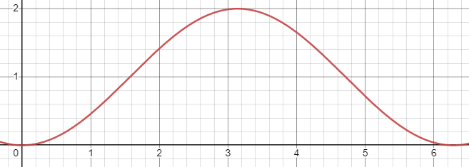
As we shall see, simple waves such as the sine wave above create "pure" sounds to our ears. The more complex sounds we hear in everyday life can be thought of as the combination, or superposition, of many different sound waves.
How Do We Represent Sound in a Computer?
The amount of pressure that a sound source creates over time is a continuous function, i.e., the pressure changes over time in a smooth fashion without any discontinuities. This is immediately a problem for us as a programmer: we can't represent continuous functions precisely in a digital computer! Why is this? If there are no discontinuities in the function because it is continuous, that means that it is infinitely divisible, i.e., for any two data points generated by the function, there always exists a point "in-between" those two points. This immediately implies that to store the result of a continuous function, we would need an infinite amount of memory. But memory is a real, physical commodity in a computer, so we can't have an infinite amount of it! (N.B., the "digital" in "digital computer" indicates this fact. All data in a computer is discrete, i.e., discontinuous, in nature!)
So what can we do? Well, rather than representing all of the values of this continuous wave, we will instead choose a finite number of samples from the wave. Each sample is a single integer describing the magnitude of the pressure at a given point in time. Below is an example of us choosing to sample the wave at every units of time to approximately .
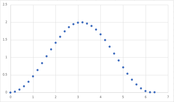
Note that this choice of the number of samples allows to approximate the shape of the continuous wave quite well. However, a different choice may not net as good of a result. For example, here's what the wave looks like if we sample at every unit of time.
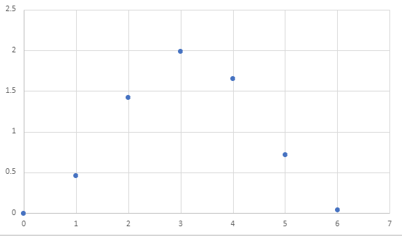
It isn't clear that our data captures a sine wave at all! When we use even more samples, e.g., units of time, it becomes very obvious we are approximating our original sine wave.

But perhaps that was overkill? We could definitely approximate the shape of the wave using less samples!
Because each sample is captured by a single integer, we must carefully choose the amount of samples we are willing to make when representing audio. More samples lead to more accurate sound, but take up more memory!
Assuming we know the sample rate, i.e., the interval at which we sample data from the sound wave, we can represent sound as a list of integers. Here are lists of integers corresponding to the three waves given above:
(define example-digital-wave
(|> (range 0 (* 2 3.14) 0.2)
(lambda (l) (map (lambda (x) (- x (/ 3.14 2))) l))))
(define example-digital-wave-less-samples
(|> (range 0 (* 2 3.14) 1)
(lambda (l) (map (lambda (x) (- x (/ 3.14 2))) l))))
(define example-digital-wave-more-samples
(|> (range 0 (* 2 3.14) 0.05)
(lambda (l) (map (lambda (x) (- x (/ 3.14 2))) l))))
(length example-digital-wave)
(list-take example-digital-wave 10)
(length example-digital-wave-less-samples)
example-digital-wave-less-samples
(length example-digital-wave-more-samples)
(list-take example-digital-wave-more-samples 10)
Characteristics of a Sound Wave
Now that we know how we'll represent digital audio (as lists of integers), we can now talk about the characteristics of a sound wave that shape how we perceive the sound. Throughout our discussion, we'll illustrate our waves as continuous functions, but remember our representation is merely an approximation of them!
The form of a wave is the shape of its repeated pattern. A sine wave, like the one above, is called so because its form follows the repetitive nature of the mathematical function. In terms of acoustic properties, the shape of the form broadly determines the timbre or quality of the sound, e.g., is it harsh or soft sounding?
In addition to the waveform, there are two other important properties of a wave that governs how we "hear" it:
-
The frequency of a wave is the number of times the waveform pattern repeats over a fixed time interval. We typically measure the frequency of a wave in hertz (Hz), repetitions per second. The frequency of a wave governs the pitch of the sound we perceive, e.g., is it a low tone or a high tone?
Alternatively, we can talk about the period of the wave: the duration of a single pattern. Note that period and frequency have an inverse relationship: frequency (patterns per second) is the inverse of period (seconds per pattern)!
-
The amplitude of a wave is the height of its largest peak. We measure the amplitude in decibels (dB), a "unitless" quantity describing the ratio between two values (on a logarithmic, base-10 scale). In terms of sound waves, this ratio is the “rest state” of the medium the wave propagates through and its peak. The amplitude of a wave governs how loud the sound is.
Thus, we can generate different kinds of sounds by varying:
- The waveform to get different sorts of tones.
- The frequency to obtain different pitches.
- The amplitude to vary the loudness of the sound.
In lab, we'll look at creating different sounds using Scheme, a process called sound synthesis!
Self Checks
Problem: Exploring Sampling Rate (‡)
As discussed in the reading, choosing the sample rate of an audio clip is an exercise in trade-offs: audio precision versus storage space. To get a concrete feel for these trade-offs, watch this video illustrating the differences in encoding audio as we vary two values:
- The sample rate as we previously discussed in the reading is how often we record values from the sound wave.
- The bit depth is the size of the range of values we capture per sample.
If a lower sample rate causes discontinuities in the axis of time, a lower bit depth causes discontinuities in the axis of pressure. With a smaller range of possible values, we cannot capture nuances between differences in pressure between samples.
- All The Sample Rates: https://www.youtube.com/watch?v=6kIHsGJSUrY
Watch the video and in your reading response, simply note the highest bit depth and sample rate where you perceive no difference in the sound relative to highest values (16 bits, 44.1 kHz sample rate). For fun, if you have a digital music collection, you might want to revisit it and see what the bit depth and sample rates of your music files are! Do you have any files that have low bit depths or sample rates? Can you tell the difference?
Waveforms
In this lab, we'll apply iteration towards manipulating audio at the waveform level!
Preparation
a. Introduce yourself to your partner, discuss strengths and weaknesses, agree upon work procedures, etc.
b. The person nearest the board is Side A. The other person is Side B. Grab the code from:
Pixel Manipulation
In this lab, we'll apply iteration towards manipulating images at the pixel level!
Preparation
a. Introduce yourself to your partner, discuss strengths and weaknesses, agree upon work procedures, etc.
b. The person nearest the board is Side A. The other person is Side B. Grab the code from:
Manipulating Waveforms
Creating Waveforms
In yesterday's lab, we learned that we represent sound waves as vectors of floating-point numbers in the range -1.0 to 1.0.
Thus, to generate sounds, we simply need to provide such a vector to the sample-node function of the audio library.
For example, we saw how to generate white noise by randomly generating either 1.0 or -1.0 for each sample:
(import audio)
; The default sample rate for sample-node is 16000 hz
(define sample-rate 16000)
(define duration 2)
(define num-samples (* sample-rate duration))
(define index->noise-sample
(lambda (i)
(- (random 3) 1)))
(let* ([samples (vector-range num-samples)])
(begin
(vector-map! index->noise-sample samples)
(sample-node samples)))
In this code snippet, we create a vector of numbers from 0 to num-samples - 1.
Think of these numbers as the index i of each sample from the sound wave.
We then transform each index into an appropriate random number by using random.
Note that we use mutation via vector-map! to avoid creating excess vectors.
If we used vector-map, we would have created an extra vector on top of the vector created by vector-range.
Since many samples are necessary to synthesize sound, e.g., 16000 * 2 = 32000 samples for a two-second clip at low-quality, it is prudent to avoid creating copies of these vectors whenever possible.
This is precisely a use case where mutation is necessary to write performant code!
Example: a square wave
We perceive tones as sound waves with patterns occurring at a particular frequency. We, therefore, can create a tone by constructing a sound wave with a regularly occurring pattern. There are a number of fundamental waveforms in digital audio.
As an example of this, let's review how we created a sound wave consisting of a square waveform from yesterday's lab. Within a single occurrence of the square waveform pattern:
- The first half of the samples are the minimum possible amplitude,
-1.0. - The second half of the samples are the maximum possible amplitude,
1.0.
Let's write a function that mutates a vector of indices into appropriate samples for a square wave.
We'll decompose this problem by writing a function that transform one index into a square wave sample and then use vector-map! to apply that function to mutate every element of our vector.
(define index->square-sample
(lambda (i total-samples)
(if (< i (/ total-samples 2))
-1.0
1.0)))
(define make-square-samples
(lambda (sz)
(let* ([samples (vector-range sz)])
(begin
(vector-map! (section index->square-sample _ sz) samples)
samples))))
(display (make-square-samples 2))
(display (make-square-samples 10))
Observe in that output that the first half vector values is -1.0 and the other half is 1.0.
Note that vector-map! expects a function of one argument which we obtain by sectioning index->square-sample, provided the intended size of the vector as the second argument.
To apply index->square-sample to create a clip that consists of many square waves, we can think of replicating a single square wave as many times as needed.
This is the role of the vector-replicate function that we wrote.
(vector-replicate n vec) creates a new vector that consists of n copies of vec joined together.
We can view this problem as a sort of mapping problem between indices of the source vector vec and the larger vector we wish to return ret.
Suppose vec is (vector "a" "b") and we want to replicate this 5 times.
The vector ret we will produce has length 5 * 2 = 10.
Let's imagine creating this vector with a call (vector-range 10) so ret initially contains the numbers 0 ... 9.
We need to map these values, i.e., indices, into valid indices of vec:
0 1 2 3 4 5 6 7 8 9
↓ ↓ ↓ ↓ ↓ ↓ ↓ ↓ ↓ ↓
"a" "b" "a" "b" "a" "b" "a" "b" "a" "b"
What function when given the top number gives you the bottom number?
It turns out this is the remainder function!
(remainder n k) returns the remainder of .
(let ([ret (vector-range 10)])
(begin
(vector-map!
(lambda (i) (remainder i 2))
ret)
ret))
In general, remainder allows us to perform "modulo" arithmetic where we want to consider numbers up
to a certain value (2 in this case) and "wrap around" when we reach either range of values.
Let's combine these two concepts to implement vector-replicate and put it together with index->square-sample to generate a square wave at 440 Hz (concert A pitch):
(import audio)
(define index->square-sample
(lambda (i total-samples)
(if (< i (/ total-samples 2))
-1.0
1.0)))
(define vector-replicate
(lambda (n vec)
(let* ([vec-len (vector-length vec)]
[sz (* n vec-len)]
[ret (vector-range sz)])
(begin
(vector-map!
(lambda (i)
(vector-ref vec (remainder i vec-len))) ret)
ret))))
(define sample-rate 16000)
(define duration 2)
(define frequency 440)
(let* ([samples-per-wave (/ sample-rate frequency)]
[waves-per-clip (* duration frequency)]
[wave (vector-range samples-per-wave)])
(begin
(vector-map!
(section index->square-sample _ samples-per-wave)
wave)
(sample-node
(vector-replicate waves-per-clip wave))))
Waveform Processing
Because our audio clips are simply vectors of floats, processing audio clips amounts to transforming these vectors of numbers, typically with vector-map!
There are many operations that we can perform over our audio clips, e.g.,
- Combine clips so that the sounds play at the same time.
- Take a single clip and modify it to have pulses, giving the effect of discrete notes between played.
- Adding effects to the clip such as echo and reverb.
As an example, we'll describe a simple technique to modify a sound clip to give it a pulse. You'll implement part of this technique for the reading question and then finish it off in lab!
ASDR Envelopes
So far, our sound waves have been continuous tones. How might we synthesize notes or pulses of sound? We can do so by applying an envelope to our wave which will control its volume. Sound envelopes are a very simple example of an effect we can apply to a wave of sound.
Recall that the amplitude of a wave determines its volume. To create the effect of a "note," we want to control the amplitude of the wave over time to simulate how the volume changes over the lifetime of a note. The standard ADSR envelope recognizes four such stages in the lifetime of a note:
- Attack: the period where the wave ramps up from zero amplitude to its peak amplitude.
- Decay: the period when the wave ramps down from its peak to a designated sustained volume.
- Sustain: the period when the wave maintains its designated sustained volume.
- Release: the period when the wave moves from its sustain level back to zero amplitude.
Here is a diagram illustrating the different portions of the ADSR envelope (from the Wikipedia article on the subject):

Relative to the sound samples, we can think of each individual point in the envelope as a multiplier. For the th sample of the sound clip, we would multiply it by the th point of the envelope to moderate its volume.
There is an art to picking appropriate values for each of these stages to create a realistic sound note. For our purposes, let's first create a simple envelope that:
- Has an instantaneous attack, i.e., the pulse starts at maximum volume.
- Has no decay or sustain; the remaining portion of the envelope releases from maximum volume back to rest.
This envelope might look like this:
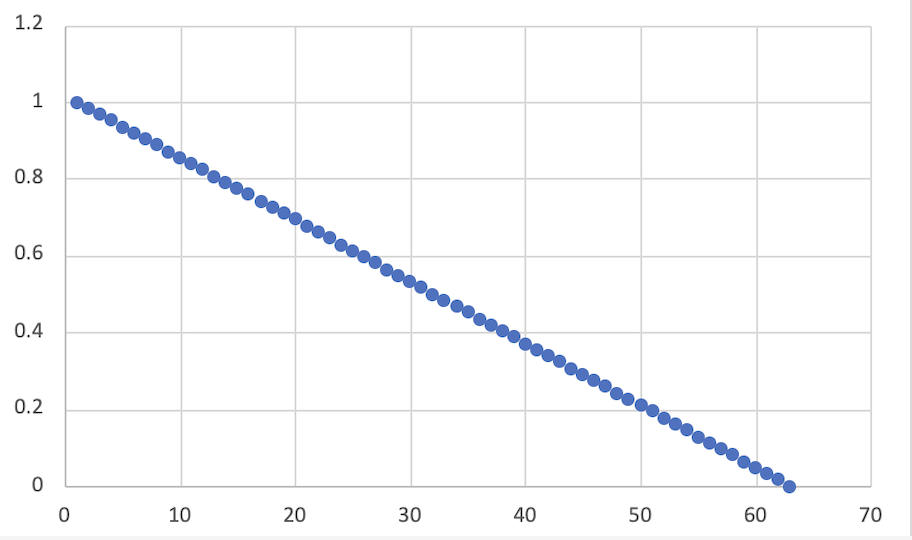
With the start of the envelope being 1.0 decreasing linearly to 0.0 by the end of the envelope.
If we take our sine wave from before:
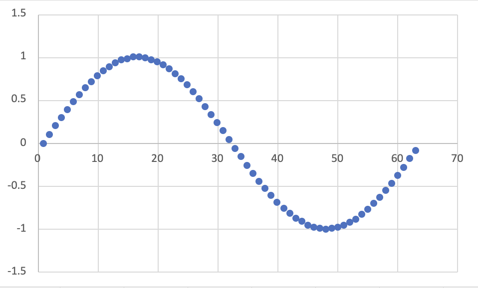
We can apply the envelope by taking the th sample and multiplying it by the th point of the envelope.
This results in a modified sine wave:
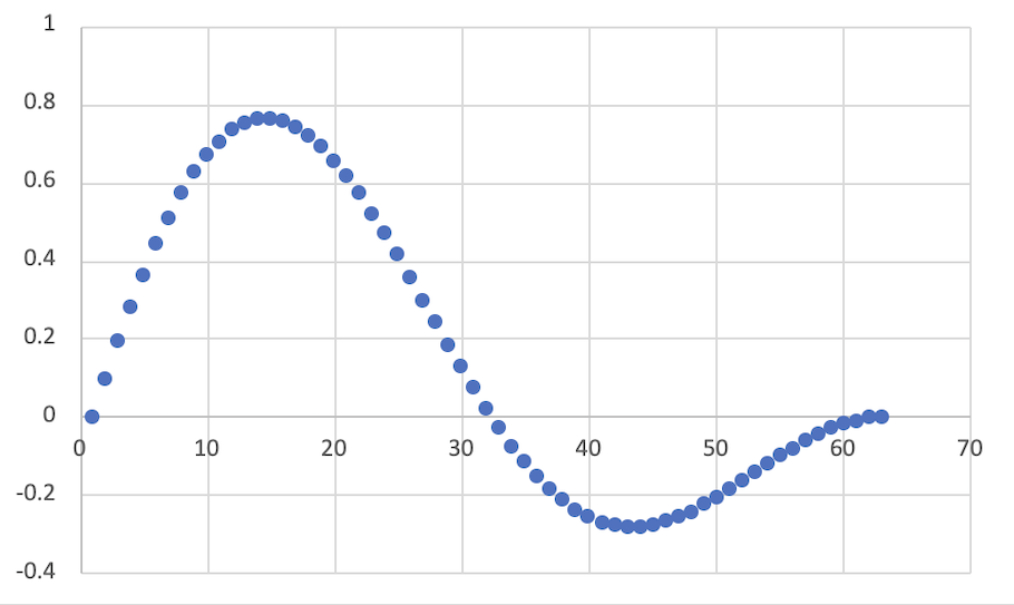
The result is a pure sine tone that is initially loud and then decays over the duration of the clip to no volume.
ASDR envelopes are a great example of the power of manipulating sound as vectors of floating-point numbers. We can do lots of interesting transformation over sounds just by applying our big-ticket operations over the samples!
Self-Checks
Problem: Making the Envelope (‡)
Create a function simple-envelope that takes total-samples, the total number of samples in the clip as input.
The function then outputs the envelope described above:
- The envelope starts at
1.0and linearly decays to0.0over its lifetime.
Here is an example of its usage for reference:
> (simple-envelope 1)
(vector 1.0)
> (simple-envelope 5)
(vector 1.0 0.8 0.6 0.4 0.2)
> (simple-envelope 10)
(vector 1 0.9 0.8 0.7 0.6 0.5 0.4 0.3 0.2 0.1)
In lab, you'll apply this function to your synthesized sounds to make notes!
Animation
So far in the course, we have outputted static images. However, we often want to produce the effect of animation in our programs, whether it is to make our user interface snazzier or build a game. In addition to animation, we may also want to have users interact with our program in natural ways, e.g., via buttons or keyboard input.
In this reading, we introduce the animation and interactivity features of Scamper so that you can build true multimedia-oriented programs!
The Canvas
All the image-rendering facilities of Scamper ultimately rely on a feature built into every modern browser, the canvas. A canvas is a user-interface element that can be drawn on, similarly to a physical canvas that an artist paints on. When we output a drawing, e.g.,
(import image) (overlay (rotate 45 (solid-square 100 "purple")) (solid-square 100 (rgb-lighter (color-name->rgb "red"))))
The drawing is ultimately rendered onto a canvas that is managed by the Scamper runtime. In other words, we never had to worry about manipulating this canvas object!
However, Scamper also allows us to manipulate canvases directly. In particular, we'll need to be able to draw on canvases in a mutating fashion in order to create the effect of animation!
The functions for manipulating canvases are found in the canvas library.
The key function here is (make-canvas width height) which makes a canvas of a given width and height.
Once a canvas is made, we can draw on it with the various functions found in the canvas library.
We can then render the canvas to the screen by displaying it.
(import canvas)
(import image)
(define canv (make-canvas 200 200))
(display canv)
(ignore
(canvas-rectangle! canv 0 0 200 200
"outline" "black"))
(ignore
(canvas-rectangle! canv 25 25 150 150
"solid" "green"))
(ignore
(canvas-circle! canv 100 100 50 "solid" "red"))
Unlike our drawing functions, the canvas drawing functions mutate the canvas by drawing a shape at a particular location.
Thus, the order of our mutating calls matters; as we see from the example above, the red circle is on top of the green square because we drew the circle after the square.
The origin of a canvas is the upper-left corner of the canvas and runs positively to the right and down.
This API for drawing is more low-level. Observe how we have to specify the location of each shape that we draw and take care to paint objects in the right order. Sometimes this trade-off is worth it, but other times, it is more convenient to use our higher-level drawing API. We can bridge this gap by creating a drawing and then asking the canvas to render it!
(import canvas)
(import image)
(define canv (make-canvas 200 200))
(display canv)
(ignore
(canvas-drawing! canv 0 0
(overlay
(outlined-square 200 "black")
(solid-circle 50 "red")
(solid-square 150 "green"))))
Animation
With our mutable canvas, we can now code up the effect of animation!
The critical function here is animate-with.
(animate-with func) takes a function as input and calls this function repeatedly at a rate of approximately 60 times per second.
This function func takes the current time in milliseconds and performs a task.
func should return #t if animate-with should continue calling it, otherwise, it should return #f which terminates this looping process.
We can use animate-with to create the effect of animation by providing a function that paints onto the canvas on every call.
For example, here is an invocation of animate-with that alternates the color of the square every second:
(import canvas)
(import image)
(define canv (make-canvas 200 200))
(display canv)
(ignore
(animate-with
(lambda (time)
(let ([color
(if (> (remainder (round time) 2000) 1000)
"blue"
"red")])
(begin
(canvas-drawing! canv 0 0
(overlay
(outlined-square 200 "black")
(solid-square 150 color)))
#t)))))
The color of the square is dependent on the time passed to the function we provide to animate-with.
Because time's unit is milliseconds, we can check to see if a second has passed by checking the remainder of the time after dividing it by 2000, i.e., 2 seconds.
This remainder computation effectively makes the timer oscillate between zero and two seconds; at this time, we simply check to see if we are in the 0–1 or 1–2 second range and pick a color based off of that.
An important note about painting on the canvas is that we do not clear the contents of the canvas automatically. We can see this by drawing an image where its position is based on the time:
(import canvas)
(import image)
(define canv (make-canvas 200 200))
(display canv)
(ignore
(animate-with
(lambda (time)
(let ([pos (remainder (round time) 200)])
(begin
(canvas-rectangle! canv 0 0 200 200 "outline" "black")
(canvas-circle! canv pos pos 25 "solid" "green")
#t)))))
Becuase the canvas's contents are not wiped on each animation frame, we "smear" the circle across the canvas! To fix this, we need to manually wipe the screen by painting over it.
(import canvas)
(import image)
(define canv (make-canvas 200 200))
(display canv)
(ignore
(animate-with
(lambda (time)
(let ([pos (remainder (round time) 200)])
(begin
; This first solid white rectangle "wipes" the canvas!
(canvas-rectangle! canv 0 0 200 200 "solid" "white")
(canvas-rectangle! canv 0 0 200 200 "outline" "black")
(canvas-circle! canv pos pos 25 "solid" "green")
#t)))))
Interactivity
We can see that all of our animations above run forever.
This is not always desirable!
However, it is not obvious how we should signal to our animation function that it should return #f instead of #t.
To do this, we'll maintain a piece of mutable state that indicates whether the animation should continue. Using a vector for this purpose is overkill because we only need a single mutable slot! Thus, we'll use a reference cell for this purpose, essentially a one-element vector with a simpler API.
(ref v)makes a reference cell initially holding the valuev.(deref r)returns the value contained in the reference cellr.(ref-set! r v)makes cellrcontain valuev.
Finally, to allow the user to toggle the state of the animation, we'll use canvas-onclick! to register a callback function with the canvas that is run whenever the canvas is clicked by the user.
This function will toggle the boolean found in the reference cell.
Once the boolean is toggled off, the animation ends!
(import canvas)
(import image)
(define continue? (ref #t))
(define canv (make-canvas 200 200))
(display canv)
(ignore (canvas-onclick! canv
(lambda () (ref-set! continue? (not (deref continue?))))))
(ignore
(animate-with
(lambda (time)
(let ([color
(if (> (remainder (round time) 2000) 1000)
"blue"
"red")])
(begin
(canvas-drawing! canv 0 0
(overlay
(outlined-square 200 "black")
(solid-square 150 color)))
(deref continue?))))))
Self-Checks
Problem: Take-off, for real! (‡)
Here is an oldie but a goodie, a rocket ship:
(import image)
(define rocket
(above
(solid-triangle 50 "green")
(solid-square 50 "blue")
(solid-square 50 "green")
(solid-triangle 50 "red")))
(display rocket)
Use a canvas and animate-with to try to create an animation where the rocket ship progresses from the bottom of the screen to the top!
As a starting point, you can try adapting the ball-animation code from above to change the -coordinate that you draw the rocket ship at in some fashion.
ADSR
In this lab, we'll continue to synthesize sound, in particular, clips that sound like notes!
Preparation
-
Introduce yourself to your partner, discuss strengths and weaknesses, agree upon work procedures, etc.
-
The person nearest the board is Side A. The other person is Side B. Grab the code from:
Animation
In this lab, we'll use our animation loop to create various fun effects!
Preparation
-
Introduce yourself to your partner, discuss strengths and weaknesses, agree upon work procedures, etc.
-
The person nearest the board is Side A. The other person is Side B. Grab the code from:
The Final Project
To conclude our semester, you will embark on a final project with 3--4 of your peers, developing a final project aligned with the themes of the course:
Requirements and Topics
In your project you will develop one or more Scheme programs to explore an area of multimedia related to your group's interests. For example, you might consider:
- Creating a collection of musical compositions around some theme that might be out of reach for a human to perform on their own.
- Creating a piece of art using multiple complex transformation over images.
- Developing a hybrid human-computer performance piece, e.g., a musical composition with Scheme performing one of the parts, or even a dance or stage performance that incorporates Scheme programs in some way.
- Building an interactive program, e.g., a game, with image and/or audio components.
- Writing a program that performs an analysis over an image, e.g., detecting the edges of an image.
- Combining art in music in a novel manner, e.g., a visualization of a sound wave.
The possibilities are endless and only limited by your imagination!
In terms of requirements, you will produce three major products:
- A software artifact, i.e., one or more Scheme programs that accomplish your goals.
- A short presentation of your work that you will deliver in the final week of the course.
- An individual reflection on your work, to be turned in by the end of the semester.
Beyond these products, we do not have specific requirements about program size, using particular libraries, etc., so that different groups have flexibility in exploring the space of digital audio. Instead, we will be coaching you through the project milestones to add in sufficient complexity and depth, in particular, with the program that you develop, so that your final work demonstrates your knowledge of the core programming concepts of the course.
Project Milestones
To ensure that you are making appropriate progress on your final project, we will have several milestones, i.e., mini-deliverables for your group to produce. We will outline the details specifics of each deliverable in subsequent milestone deliverable write-ups.
- Milestone #1 (Friday 11/15): groups are formed and project topic brainstorming begins.
- Milestone #2 (Friday 11/22): identification of a topic for the project and an architectural outline of the program(s) you will need.
- Milestone #3 (Monday 12/2): decomposition of the program outline into functions and a partially-completed program.
- Milestone #4 (Tuesday 12/10): software artifact and project presentation is due.
- Milestone #5 (Friday 12/13): individual reflections are due.
Final Deliverables
The final deliverables consist of three artifacts:
- One or more Scheme programs that address the problems you wish to solve. The programs should be complete and well-formatted according to the course style guides.
- A presentation no more than 8 minutes in length giving an overview of your work along with a demo or performance. You will produce a slide deck for this presentation and turn it in. Be prepared to answer questions from the audience.
- A short reflection on your work describing the problem you solved, your specific contributions to the project, and a bug that you personally encountered in your project and how you fixed it. These reflections will be completed individually and will reflect each individual's contribution to the overall project.
Final Reflection
Your final project grade will come primarily from your final reflection paper for the course. Note that the final reflection is an individual deliverable. You should work independently on your reflection so that the writing reflects your interpretation of your project. You should not collaborate with your group members on any part of this reflection! Furthermore, you should not use a large language model, e.g., ChatGPT, to help you author your reflection in part or whole.
Your final reflection should be a written paper meeting the following specifications:
- PDF format.
- At least 500 words and no more than 750 words in length.
- 1" margins, 12 pt font, double-spaced.
Your reflection must include the following four parts:
- Overview. Give a brief overview of your project in your own words: what did you build and why?
- Architecture. Give a brief overview of your project's architecture: how did your group break down the problem into components?
- Your Contributions. Give a description of your contributions to the project: which components did you contribute code to and how much code did you contribute to each?
- Bug Log. Give a description of a bug that you personally encountered during development and how you systematically solved the issue. (More requirements below.)
Overview, Architecture, and Contribution sections should be in paragraph form.
In the Bug Log, you are encouraged to use a mix of paragraphs and numbered steps to best communicate your process. Your Bug Log should answer the following questions:
- What did you initially observe that indicated a bug was present?
- How did you fix the bug? You should describe the bug-fixing process as a cycle of the following two steps until a solution was found:
- What steps did you take to understand and diagnose the issue?
- What did you do to fix the bug? Did it succeed?
- In hindsight, what should you have done to avoid introducing the bug in the first place?
To answer this question, you should choose a bug of substantial breadth and difficulty that you required multiple attempts of the "diagnose/fix" cycle to address the bug. Such bugs should be logic errors, i.e., bugs that arise because your strategy to solve a problem was wrong, not because you mistyped a construct.
Grading
Our goal is that if you do the work and follow good habits, you should get at least an M.
There are no redos available for this project.
-
Excellent:
- Project code is high quality both in terms of functionality (i.e., the code accomplishes the task at hand) and style.
- Project presentation covers all of the required points, involves everyone in the group, and stays within time budget.
- Personal reflection is high quality, covering all required points and is evident of reflection on the software development process.
-
Meets expectations:
- Project code is functional (i.e., the code accomplishes the task at hand) but may have some bugs or substantial style issues due to lack of revision.
- Project presentation covers all of the required points.
- Personal reflection covers all the required points but does not discuss them at sufficient depth.
Self-Checks
Problem: Brainstormin' (‡)
Brainstorm no less than three project ideas for your final project. Make sure to bring your ideas to class to share them with your group!
Take-home assessment 8: Pixel problems
We consider a variety of mechanisms for manipulating images according to their pixels.
Name your file for this assignment pixel-problems.scm. Please make sure to begin with the starter code.
Background
As you may recall from your recent work, we can envision each image as a width-by-height grid of colored "pixels". We call such a structure a "bitmap". As you might expect, each pixel in the grid is indexed by a column and a row. Here's a diagram of the indices in a w-by-h bitmap.
0 1 2 3 w-2 w-1
+-----+-----+-----+-----+- .... -+-----+-----+
0 | 0,0 | 1,0 | 2,0 | 3,0 | |w-2,0|w-1,0|
| | | | | | | |
+-----+-----+-----+-----+- .... -+-----+-----+
1 | 0,1 | 1,1 | 2,1 | 3,1 | |w-2,1|w-1,1|
| | | | | | | |
+-----+-----+-----+-----+- .... -+-----+-----+
2 | 0,2 | 1,2 | 2,2 | 3,2 | |w-2,2|w-1,2|
| | | | | | | |
+-----+-----+-----+-----+- .... -+-----+-----+
| . | . | . | . | | . | . |
. . . . . .
| . | . | . | . | | . | . |
+-----+-----+-----+-----+- .... -+-----+-----+
h-2 |0,h-2|1,h-2|2,h-2|3,h-2| |w-2, |w-1, |
| | | | | | h-2 | h-2 |
+-----+-----+-----+-----+- .... -+-----+-----+
h-1 |0,h-1|1,h-1|2,h-1|3,h-1| |w-2, |w-1, |
| | | | | | h-1 | h-1 |
+-----+-----+-----+-----+- .... -+-----+-----+
You'll note that columns run from 0 to w-1 and rows run from 0 to h-1.
We can turn a bitmap into a single w*h vector of pixels by putting each row next to the previous one.
0 1 2 w-1 w w+1 w+w-1 w+w w+w+1
+-----+-----+-----+- .... -+-----+-----+-----+- .... -+-----+-----+-----+- ...
| 0,0 | 1,0 | 2,0 | |w-1,0| 0,1 | 1,1 | |w-1,1| 0,2 | 1,2 |
+-----+-----+-----+- .... -+-----+-----+-----+- .... -+-----+-----+-----+- ...
As you may be able to tell, the pixel at position (c,r) can be found at (+ c (* r w)).
Scamper provides two primary procedures that permit us to convert between images and vectors of RGB colors.
;;; (image->pixels img) -> canvas? ;;; img: canvas? ;;; Returns a vector of rgb values corresponding to the pixels of the given canvas. ;;; ;;; (pixels->image pixels width height) -> canvas? ;;; pixels: vector? of rgb values ;;; width: integer? ;;; height: integer? ;;; Returns a new canvas with the given pixels and dimensions width × height.
Part one: Setting rows and columns
Let's begin our exploration of bitmaps by working on individual rows and columns of the image.
Problem 1a.
Write the following procedure:
;;; (set-row! pixels width height row color) -> void?
;;; pixels : (all-of (vector-of rgb?) (has-length (* width height)))
;;; width : positive-integer? (represents the width of the image)
;;; height : positive-integer? (represents the height of the image)
;;; row : non-negative integer?
;;; color : rgb?
;;; Sets the given row of the image to the specified color.
(Hint: Write a helper procedure that recurses over the column under consideration.)
Problem 1b.
Write the following procedure.
;;; (set-rows! pixels width height top bottom color) -> void?
;;; pixels : (all-of (vector-of rgb?) (has-length (* width height)))
;;; width : positive-integer? (represents the width of the image)
;;; height : positive-integer? (represents the height of the image)
;;; top : non-negative integer?
;;; bottom : non-negative integer?
;;; color : rgb?
;;; Sets the rows between top (inclusive) and bottom (exclusive)
;;; to the given color.
(Hint: Write a helper procedure that recurses over the rows, calling
set-row! for each row.)
(Note: Do not set the final row.)
Problem 1c.
Write the following procedure.
;;; (set-column! pixels width height column color) -> void?
;;; pixels : (all-of (vector-of rgb?) (has-length (* width height)))
;;; width : positive-integer? (represents the width of the image)
;;; height : positive-integer? (represents the height of the image)
;;; column : non-negative integer?
;;; color : rgb?
;;; Sets the given column of the image to the specified color.
(Hint: Write a helper procedure that recurses over the column.)
Problem 1d.
Write the following procedure.
;;; (set-columns! pixels width height left right color) -> void?
;;; pixels : (all-of (vector-of rgb?) (has-length (* width height)))
;;; width : positive-integer? (represents the width of the image)
;;; height : positive-integer? (represents the height of the image)
;;; left : non-negative integer?
;;; right : non-negative integer?
;;; color : rgb?
;;; Sets the columns between left (inclusive) to right (exclusive)
;;; to the given color.
(Hint: Write a helper procedure that recurses over the column, calling set-column! for each column.)
(Note: Once again, make sure not to include the final column.)
Problem 1e.
Write the following procedure.
;;; (set-region! pixels width height left right top bottom color) -> void?
;;; pixels : (all-of (vector-of rgb?) (has-length (* width height)))
;;; width : positive-integer? (represents the width of the image)
;;; height : positive-integer? (represents the height of the image)
;;; left : non-negative integer?
;;; right : non-negative integer?
;;; top : non-negative integer?
;;; color : rgb?
;;; Set a rectangular region of the image to `color`. The region is
;;; bounded on the left by `left` (inclusive), on the right by `right`
;;; (exclusive), on the top by `top`, and on the bottom by `bottom`.
(Hint: You should be able to write set-region! with a relatively minor modification to either set-rows! or set-columns! and its helpers.)
Part two: Modifying images
Once we can directly access and modify pixels in an image, we also have the opportunity to write more complex image transformations, including transformations based on the position. Let's start with a somewhat silly one.
Write a procedure, (positionally-transform-pixels! pixels width height), that takes a vector of pixels representing a width-by-height image as a parameter and modifies each pixel by using the following procedure.
;;; (positionally-transform-pixel color col row) -> rgb?
;;; color : rgb?
;;; col : nonnegative-integer?
;;; row : nonnegative-integer?
;;; Transform `color` based on its column and row.
(define positionally-transform-pixel
(lambda (color col row)
(rgb (+ (rgb-red color)
(remainder (round (sqrt (+ (sqr (- col 50)) (sqr (- row 50)))))
64))
(+ (rgb-green color)
(* 2 (remainder (round (sqrt (+ (sqr (- col 150)) (sqr (- row 50)))))
32)))
(+ (rgb-blue color)
(* 3 (remainder (round (sqrt (+ (sqr (- col 200)) (sqr (- row 200)))))
25)))
(rgb-alpha color))))
Hint: Think about how to decompose the problem. You will likely find it helpful to write helper procedures (e.g., that process a row or a column).
Once you've written positionally-transform-pixels!, you can see its effect on an image with the following procedure.
;;; (positionally-transform img) -> image?
;;; img : image?
;;; Transform an image by adding the column of each pixel to its red
;;; component, the row of each pixel to its blue component, and the
;;; average of the row and column to the green component.
(define positionally-transform
(lambda (img)
(let ([pixels (image->pixels img)])
(positionally-trasform-pixels! pixels)
(pixels->image pixels (image-width img) (image-height img)))))
Let's see how it works.
> (positionally-transform (solid-square 300 "gray"))

> (positionally-transform (solid-circle 300 "black"))
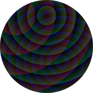
> (positionally-transform (overlay (solid-circle 300 "black")
(solid-square 300 "gray")))
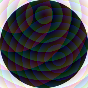
> (positionally-transform kitten)

Part three: Steganography
Steganography is a technique for hiding information within a larger corpus. For example, some people conceal messages in letters by using, say, each fifth letter in the original message to represent a new message. (I'm not talented enough to give an example.)
Since our eyes can't always distinguish nearby colors, images can often be a good host for hidden information; we modify the image to add information at each pixel, or each few pixels.
Here's one approach for doing so: We develop a mechanism for converting the sum of components in each pixel to a letter. To hide a message in an image, we then convert each pixel so that it has the right sum.
We'll use a simple mapping of letters to the numbers 0, ..., 31.
- 0: end of message
- 1: a
- 2: b
- 3: c
- 4: d
- 5: e
- ...
- 20: t
- 21: u
- 22: v
- 23: w
- 24: x
- 25: y
- 26: z
- 27: period
- 28: space
- 29: newline
- 30: reserved for future use; do not use (appears as underscore)
- 31: anything else (appears as asterisk)
How do we convert the components to a number? We can add them up then take the remainder when divided by 32.
;;; (color->number color) -> integer?
;;; color : color?
;;; Use the not-so-secret formulat to convert a color to an appropriately
;;; representative integer.
(define color->number
(lambda (color)
(remainder (+ (rgb-red color) (rgb-green color) (rgb-blue color))
32)))
Suppose we want to encode the word "cat" in our image, and that the first four pixels in the image are (rgb 255 100 10), (rgb 255 100 255), (rgb 255 100 10), and (rgb 100 200 128). The sum of the components in the first pixel are 365. (remainder 365 32) is 13. We want it to be 3 (the letter c). So we need to subtract ten from the components. Perhaps we use (rgb 248 98 9). Let's check.
> (color->number (rgb 248 98 9))
3
We could also have used (rgb 255 90 10) or (rgb 251 97 7) or any other way of subtracting ten.
> (color->number (rgb 255 90 10))
3
> (color->number (rgb 245 100 10))
3
> (color->number (rgb 251 97 7))
3
On to the next pixel.
> (color->number (rgb 255 100 255))
2
That one's pretty close. We want a remainder of 1 for an a. So we can convert the color to (rgb 254 100 255).
> (color->number (rgb 254 100 255))
1
The next pixel is the same color, which gives a remainder of 2. We need to get it all the way to 20 for a t. So we could add 18 to the 100 and use (rgb 255 118 255).
> (color->number (rgb 255 118 255))
20
Alternately, we could subtract 14 (perhaps 6 from the red, 2 from the green, and 6 from the blue).
> (color->number (rgb 249 98 249))
20
How do we decide whether to add or subtract? There are many strategies. Since we have to subtract from white and we have to add to black, it might be easiest to subtract from colors whose components sum to more than 127x3 and add to colors whose components sum to less than that.
Here's one strategy, which uses randomness to encode the letter in a color.
;;; (encode-letter color) -> color?
;;; letter : char?
;;; color : color?
;;; Encode a letter in a color, creating a nearby color.
(define encode-letter
(lambda (letter color)
(let* ([current (color->number color)]
[target (letter->number letter)]
[pos-diff (remainder (+ 32 (- target current)) 32)]
[r (color-red color)]
[g (color-green color)]
[b (color-blue color)]
[a (color-alpha color)]
[goal (+ r g b pos-diff)])
(if (> (+ r g b) (+ 1 (* 3 127)))
(color-decrement-to r g b a (+ -32 goal))
(color-increment-to r g b a goal)))))
;;; (color-decrement-to r g b a target) -> color?
;;; r : rgb-component?
;;; g : rgb-component?
;;; b : rgb-component?
;;; a : rgb-component?
;;; target : (all-of exact-integer? (at-least 0) (at-most (+ r g b)))
;;; Randomly decrement `r`, `g`, and `b` until we reach a sum of `target`.
(define color-decrement-to
(lambda (r g b a target)
(let ([rgb-sum (+ r g b)])
(if (= rgb-sum target)
(rgb r g b a)
(let ([rand (random rgb-sum)])
(cond
[(< rand r)
(color-decrement-to (- r 1) g b a target)]
[(< rand (+ r g))
(color-decrement-to r (- g 1) b a target)]
[else
(color-decrement-to r g (- b 1) a target)]))))))
;;; (color-increment-to r g b a target) -> color?
;;; r : rgb-component?
;;; g : rgb-component?
;;; b : rgb-component?
;;; a : rgb-component?
;;; target : (all-of nonnegative-integer? (at-most (* 3 255)) (at-least (+ r g b)))
;;; Randomly increment `r`, `g`, and `b` until we reach a sum of `target`.
(define color-increment-to
(lambda (r g b a target)
(let ([rgb-sum (+ r g b)])
(if (= rgb-sum target)
(rgb r g b a)
(let ([rand (random (- (* 3 255) rgb-sum))])
(cond
[(< rand (- 255 r))
(color-increment-to (+ r 1) g b a target)]
[(< rand (+ (- 255 r) (- 255 g)))
(color-increment-to r (+ g 1) b a target)]
[else
(color-increment-to r g (+ b 1) a target)]))))))
Let's give it a try.
> (rgb->string (encode-letter #\t (rgb 255 100 255)))
"250/97/249"
> (rgb->string (encode-letter #\t (rgb 255 100 255)))
"248/99/249"
> (rgb->string (encode-letter #\t (rgb 255 100 255)))
"246/98/252"
> (color->number (rgb 250 97 249))
20
> (color->number (rgb 248 99 249))
20
> (color->number (rgb 246 98 252))
20
Great. We have a procedure that lets us encode letters. One fewer step in the bigger picture.
Where were we? Oh, that's right. We were encoding the word "cat". We've done the first three letters.
Last up is the "end of message" value, 0. Let's see what value the current color gives.
> (color->number (rgb 100 200 128))
12
As always, there are many possible colors. We'll go with (rgb 96 196 124).
> (color->number (rgb 96 196 124))
0
We're done. At least we're done with the example. Now it's time to write some helpful procedures.
Problem 3a.
You may note that encode-letter requires a helper procedure, letter->number. Write at least three additional tests for letter->number and then implement it.
> (letter->number #\b)
2
> (letter->number #\nul)
0
> (letter->number #\space)
28
> (letter->number #\.)
27
> (letter->number #\?)
31
> (letter->number #\!)
31
Problem 3b.
Document, write at least three additional tests for, and implement a procedure, (color->letter color), that uses the "add the components, take the remainder, look it up in the table above" approach to find the letter that corresponds to a color. (You can use #\nul for "end of input".)
> (color->letter (rgb 0 0 0))
#\nul
> (color->letter (rgb 33 0 0))
#\a
> (color->letter (rgb 32 (+ 32 27) 0))
#\.
> (color->letter (rgb 32 64 (+ 128 28)))
#\space
> (color->letter (rgb 32 64 (+ 128 29)))
#\newline
> (color->letter (rgb 32 64 (+ 128 30)))
#\_
> (color->letter (rgb 32 64 (+ 128 31)))
#\*
Problem 3c.
Document and write a procedure, (extract-text pixels), that takes a vector of colors as input, reads all the letters (using color->letter) until it hits #\null, and then puts them together into a string. If there's no #\null,
> (extract-text (list->vector (map (lambda (x) (rgb x 0 0))
(range 1 65))))
"abcdefghijklmnopqrstuvwxyz. \n_*"
> (extract-text (vector (rgb 1 1 1) (rgb 0 1 0) (rgb 5 5 10)
(rgb 8 8 16)))
"cat"
> (extract-text (list->vector (map (lambda (x) (rgb x x x)) (range 1 10))))
Runtime error [...]: (vector-ref) vector-ref: index 9 out of bounds of list
; We never hit a zero, so this crashes. That's okay. You could also stop
; at the end of the vector.
Problem 4d.
Document and write a procedure, (steg-decode img), that takes an image as an input and "decodes" hidden text using extract-text.
> (steg-decode (overlay (solid-circle 10 "black")
(solid-square 10 (rgb 1 0 0))))
"aaa"
Problem 5e.
Document and write a procedure, (insert-text! text pixels), that takes a string and vector of colors as input and updates the colors in pixels so that they encode the text.
> (define example (make-vector 6 (rgb 0 0 255)))
> (insert-text! "cat" example)
> (vector-map rgb->string example)
'#("1/3/255" "0/2/255" "7/14/255" "1/0/255" "0/0/255" "0/0/255")
; Note that we changed *four* colors. We needed to insert the null, too
> (extract-text example)
"cat"
> (let ([aphorism (make-vector 128 (rgb 128 128 128))])
(insert-text! "there is more to life than computer science." aphorism)
(extract-text aphorism))
"there is more to life than computer science."
You may assume that (vector-length pixels) is larger than (string-length text).
Problem 5f.
Document and write a procedure, (steg-encode text img), that takes a string and an image as input and "encodes" the text in the image using the specified technique. steg-encode should return a new image.
> (steg-decode (steg-encode "there is more to life than computer science"
(solid-circle 20 "blue")))
"there is more to life than computer science"
Wasn't that fun?
Grading rubric
Redo or above
Submissions that lack any of these characteristics will get an N.
- Displays a good faith attempt to complete every required part of the assignment.
Meets expectations or above
Submissions that lack any of these characteristics but have all the prior characteristics will get an R.
- Includes the specified file,
pixel-problems.scm. - Includes an appropriate header on all submitted files that includes the course, author, etc.
- Correctness
- Code runs without errors.
- Core functions are present and correct (except for non-obvious corner cases, when present)
- Part 1
(set-row! pixels width height row color)(set-rows! pixels width height top bottom color)(set-column! pixels width height column color)(set-columns! pixels width height left right color)(set-region! pixels width height left right top bottom color)
- Part 2
(positionally-transform-pixels! pixels width height)(positionally-transform img)
- Part 3
(letter->number ch)(color->letter (rgb 0 0 0))(extract-text pixels)
- Part 1
- Extended functions are present (but may not be correct):
- Part 3
(steg-decode img)(insert-text! text pixels)(steg-encode text img)
- Part 3
- Design
- Documents and names all core procedures correctly.
- Code generally follows style guidelines.
Exemplary / Exceeds expectations
Submissions that lack any of these characteristics but have all the prior characteristics will get an M.
- Correctness
- At least three tests present for each of
letter->numberandcolor->letter steg-decodeandsteg-encoderoundtrip properly, i.e., encoding a message in an image and then decoding results in the same message.
- At least three tests present for each of
- Design
- Function documentation is complete and appropriately evocative of each function's behavior.
- Code follows style guidelines completely, with at most three minor errors present.
- Code is well-designed, avoiding repeated work through decomposition and appropriate language constructs.
A Simple Synthesizer
For this mini-project, you will continue extending the basic synthesizer you developed last week into a more full-featured synthesizer. In particular, you'll implement two features:
- Multiple voices in the synthesized output, i.e., creating a wave by combining two input waves in a uniform manner.
- A complete ASDR envelope filter, building the simple envelope you developed in lab.
With these features, we are getting closer to emulating how real synthesizers work, such as the legendary Minimoog Model-D. Note in the picture of the Model-D the collections of dials for the "Oscillator Bank" and "Modifiers." These control the voices produced by the Moog as well as the ASDR envelope the Moog uses to shape its sound!
As a starting point, you should use the synthesize-square-wave-note function from your ASDR lab and their associated helper functions.
And their associated helper functions.
Note that you will be expected to use these functions as a basis for your mini-project.
Feel free to edit and modify them as you see fit to achieve the functionality described below.
Because you are using code that you used from your previous work, you should cite yourself and your partner to be clear where your code came from. In a comment at the top of your file give a brief acknowledgement describing what code you have adapted from the lab and who worked on it. The format of these acknowledgements is less important than ensuring that you write some acknowledgement in your file!
Write your program in a file called synthesizer.scm and submit it to Gradescope when you are done.
Part 1: Multi-voice synthesis
We saw that the various fundamental waveforms produce different timbre of sound.
One way to create even more varied timbres is to mix together different waveforms at different frequencies together into a single clip.
In the lab, your synthesize-square-note function generated a note from a square wave.
For this part, generalize synthesize-square-note to generate-note.
generate-note has the same parameters as synthesize-square-note—sample-rate, frequency, duration—but instead of generating a note from a square wave, it generates a note by combining a square wave and a sine wave.
To generate the sine wave portion of the clip, you should leverage your lab code for making a sine wave appropriately. If you have done so, feel free to include the code in your assessment verbatim with appropriate acknowledgement at the top of your file. If you have not done so, you should create such functionality for this part.
To perform this superposition of waves, each sample generate-note creates is the result pointwise averaging the samples from a square wave and sine wave.
That is, the first samples from the square and sine wave are averaged together, then the second samples of each clip are averaged together, and so forth.
The resulting values, by the nature of averaging, will be valid amplitude values in the range (-1.0, 1.0).
Part 2: The ADSR Envelope
In lab, our volume envelope was a simple envelope that had an instantaneous attack and no sustain or decay. Let's enhance our envelope to a true ADSR envelope that allows you to customize the attack, sustain, decay, and subsequent release. For reference, here is the shape of an ADSR envelope from Wikipedia:
The way that we'll proceed is to specify the durations of the first three periods of the envelope, attack, sustain, and decay, with the fourth period, release, being implied by the first three periods.
Augment generate-note to also take a list of three floating point numbers in the range 0.0 to 1.0 that represent the relative percentages of time that the envelope, attack, and sustain should take; the release takes up the remaining time.
For example, if we pass the list (list 0.1 0.3 0.2), then the envelope should have:
- An attack period that lasts
0.1of the samples of the envelope, - A decay period that lasts
0.3of the samples, - A sustain period that lasts
0.2of the samples, and - A release period that lasts
1.0 - 0.1 - 0.3 - 0.2 = 0.4of the samples.
To create this generalized envelope, break up the envelope into its pieces:
- An attack period that increases linearly from 0.0 to 1.0.
- A decay period that decreases linearly from 1.0 to 0.5.
- A sustain period that stays at 0.5.
- A release period that decreases linearly from 0.5 to 0.0.
For reference, note that our original envelope from synthesize-square-note can be obtained by passing (list 0.0 0.0 0.0) for the envelope list.
Notes On Style
For this mini-project, we are being less specific about how you approach the tasks at hand because there are a variety of ways to approach these problems. We're concerned less about how you approach a problem, but whether your implementation reads like the solution you intend to write down. When in doubt, follow our basic principles for style:
- Make sure your code is indented correctly and employs good names for its variables.
- Realize the decomposition of the problem at hand directly using functions and let-binding to capture relevant sub-computations as necessary.
- Use top-level definitions, functions, and let-bindings to eliminate redundancy in your program.
Grading rubric
Redo or above
Submissions that lack any of these characteristics will get an N.
- Displays a good faith attempt to complete every required part of the assignment.
Meets expectations or above
Submissions that lack any of these characteristics but have all the prior characteristics will get an R.
- Includes the specified file,
synthesizer.scm. - Includes an appropriate header on all submitted files that includes the course, author, etc.
- Correctness
- Code runs without errors.
- Core functions are present and correct (except for non-obvious corner cases, when present)
-
(generate-note sample-rate frequency asdr-params). (Note:asdr-paramsmay not be present if part 2 is not fully implemented). generate-noteappropriately combines a square and sine wave.
- Design
- Documents and names all core procedures correctly.
- Code generally follows style guidelines.
Exemplary / Exceeds expectations
Submissions that lack any of these characteristics but have all the prior characteristics will get an M.
- Correctness
generate-notetakes anasdr-paramsparameter and successfully applies to create an ADSR envelope.
- Design
- Function documentation is complete and appropriately evocative of each function's behavior.
- Code follows style guidelines completely, with at most three minor errors present.
- Code is well-designed, avoiding repeated work through decomposition and appropriate language constructs.
Data abstraction
At this point in your career, you have already used a wide variety of types, including characters, strings, symbols, numbers (all sorts of numbers), and images. You've also learned a few mechanisms for grouping data together, including lists, maps, vectors, and files.
As you may have realized, you've reached the point that you can probably write your own data types, or at least something like your own data types. That is, you can find ways to structure data in a clear and coherent way and provide access to those data.
Let's explore some ways to do so.
A sample data type: Names
Well start with might seem like a comparatively simple starting point: names. In the US, most names traditionally have three basic components: a given name (also known as a first name), a middle name, and a family name (also known as a surname or last name). Some names also have a suffix, such as "Jr." or "III". A few names have prefixes, such as "King" or "Pope". (Interestingly, names with prefixes often lack middle and last names, although they may have suffixes.)
As we said, these are comparatively simple. As you design data types, you'll find that each has some complexity.
What might we do with names? We should be able to
- Construct them from the component parts.
- Extract the component parts.
- Convert them into a string for output.
- Compare two of them for sorting or similar activities.
- Determine if a value is a name.
That seems like a good starting point. Let's write the documentation for each of these.
We'll start with the basic constructor.
;;; (name prefix given middle family suffix) -> name? ;;; prefix : string? or #f ;;; given : string? ;;; middle : string? or #f ;;; family : string? or #f ;;; suffix : string? or #f
Why did we say "or #f"? Because the prefix, middle name, family name, and suffix are all optional. (All of them? Yes. There are people with only one name, including Madonna, Prince, and the computer scientist Simon.)
What should we do next? Let's see ... document, then write tests. Can
we write tests for name? Probably not until we've described a
few more procedures, but we can at least try some based on the output
type. We'll want to create a variety of forms of names.
(define ada (name "Countess" "Ada" "Augusta" "Byron" #f)) ; Perhaps "Lady Ada August King, Countess Lovelace" ; Our name model is insufficiently deep. (define babbage (name #f "Charles" #f "Babbage" #f)) (define clay (name #f "Roy" #f "Clay" "Sr")) (define hopper (name #f "Grace" "Murray" "Hopper" #f)) ; We don't normally include titles for Americans. (define qe2 (name "Queen" "Elizabeth" #f #f "II")) (define simon (name #f "Simon" #f #f #f)) (test-case "Admiral Grace Murray Hopper" equal? #t (lambda () (name? hopper))) (test-case "Charles Babbage" equal? #t (lambda () (name? babbage))) (test-case "Countess Ada Augusta Byron" equal? #t (lambda () (name? ada))) (test-case "QEII" equal? #t (lambda () (name? qe2))) (test-case "Roy Clay Sr." equal? #t (lambda () (name? clay))) (test-case "Simon" equal? #t (lambda () (name? simon)))
As long as we've referenced the name? predicate, we should document
it.
;;; (name? val) -> boolean? ;;; val : any? ;;; Determine if val is a name.
What about the tests for the name? predicate? We've effectively written
those above.
Okay, let's think about the components. We should be able to extract each of the components.
;;; (name-prefix name) -> string? or #f ;;; name : name? ;;; Get the prefix of a name. Returns #f if the name has no prefix. ;;; (name-given name) -> string? ;;; name : name? ;;; Get the given name from a name. ;;; (name-middle name) -> string? or #f ;;; name : name? ;;; Get the middle name from a name. Returns #f if the name does ;;; not contain a middle name. ;;; (name-family name) -> string? or #f ;;; name : name? ;;; Get the family name from a name. Returns #f if the name lacks ;;; a family name. ;;; (name-suffix name) -> string? or #f ;;; name : name? ;;; Get the suffix from a name. Returns #f if the name lacks a ;;; suffix.
And some tests!
(test-case "ada/prefix" equal? "Countess" (lambda () (name-prefix ada))) (test-case "ada/given" equal? "Ada" (lambda () (name-given ada))) (test-case "ada/middle" equal? "Augusta" (lambda () (name-middle ada))) (test-case "ada/family" equal? "Byron" (lambda () (name-family ada))) (test-case "ada/suffix" equal? #f (lambda () (name-suffix ada))) ; ...
You get the idea.
At this point, you're probably saying "But where's the implementation?" I'd prefer to document the remaining procedures, but I suppose we can move on to the implementation.
Implementing names
But how should we implement names? There are so many options. We
could use five-element lists. We could use five-element vectors.
We could use dictionaries indexed by the strings "prefix", "given",
"middle", "family", and "suffix". We could use strings with the
elements separated by commas or tildes or vertical bars or something
else. We could use Scheme's structs, but we don't know those
yet. So many options!
Let's choose the "obvious" one: Lists. After all, it's what we would have used a week or two ago.
Let's go!
(define name
(lambda (prefix given middle family last)
(list prefix given middle family last)))
Wasn't that fun? I suppose we could also have written the following since it accomplishes the same thing.
(define name list)
However, the first version ensures that name is always called with
five parameters.
If we're ensuring the correct number of inputs, we could also ensure that those parameters are of the correct type.
(define name
(let ([string-or-false?
(lambda (val)
(or (string? val) (equal? val #f)))])
(lambda (prefix given middle family suffix)
(cond
[(not (string-or-false? prefix))
(error (string-append "name: Invalid prefix: " prefix))]
[(not (string? given))
(error (string-append "name: Invalid given name: " given))]
[(not (string-or-false? middle))
(error (string-append "name: Invalid middle: " middle))]
[(not (string-or-false? family))
(error (string-append "name: Invalid family: " family))]
[(not (string-or-false? suffix))
(error (string-append "name: Invalid suffix: " suffix))]
[else
(list prefix given middle family suffix)]))))
Whoops. Perhaps that was too much. Oh well. It's a good strategy.
And it will help us move on to the name? predicate.
(define name?
(let ([string-or-false?
(lambda (val)
(or (string? val) (equal? val #f)))])
(lambda (val)
(and (list? val)
(= 5 (length val))
(string-or-false? (list-ref val 0))
(string? (list-ref val 1))
(string-or-false? (list-ref val 2))
(string-or-false? (list-ref val 3))
(string-or-false? (list-ref val 4))))))
And yes, name and name? together pass all the tests.
On to the other procedures. They are comparatively easy to define.
(define name-prefix (lambda (n) (list-ref n 0))) (define name-given (lambda (n) (list-ref n 1))) (define name-middle (lambda (n) (list-ref n 2))) (define name-family (lambda (n) (list-ref n 3))) (define name-suffix (lambda (n) (list-ref n 4)))
These also pass our tests.
Changing our implementation
I don't know about you, but at some point, I worry about all of those
list-refs and such. They aren't that inefficient, but they do require
a bit of extra work. Maybe we should use a vector.
Let's see ... The name procedure won't be much different.
(define name
(let ([string-or-false?
(lambda (val)
(or (string? val) (equal? val #f)))])
(lambda (prefix given middle family suffix)
(cond
[(not (string-or-false? prefix))
(error (string-append "name: Invalid prefix: " prefix))]
[(not (string? given))
(error (string-append "name: Invalid given name: " given))]
[(not (string-or-false? middle))
(error (string-append "name: Invalid middle: " middle))]
[(not (string-or-false? family))
(error (string-append "name: Invalid family: " family))]
[(not (string-or-false? suffix))
(error (string-append "name: Invalid suffix: " suffix))]
[else
(vector prefix given middle family suffix)]))))
Nor will the name? procedure. In fact, we can even take advantage
of the other procedures we would write.
(define name-prefix (lambda (v) (vector-ref v 0)))
(define name-given (lambda (v) (vector-ref v 1)))
(define name-middle (lambda (v) (vector-ref v 2)))
(define name-family (lambda (v) (vector-ref v 3)))
(define name-suffix (lambda (v) (vector-ref v 4)))
(define name?
(let ([string-or-false?
(lambda (val)
(or (string? val) (equal? val #t)))])
(lambda (val)
(and (vector? val)
(= 5 (vector-length val))
(string-or-false? (name-prefix val))
(string? (name-given val))
(string-or-false? (name-middle val))
(string-or-false? (name-family val))
(string-or-false? (name-suffix val))))))
And yes, this implementation passes all the tests. At least it did once I fixed some bugs.
Never satisfied: Yet another implementation
Are we done yet? No. We might decide that we want some practice with
maps and want to implement names with an association list. As
noted earlier, we can use strings such as "prefix" and "middle" for the keys. Let's see
what we might do. I'd suggest only putting part of the name in the
association list if it's not false.
In this case, we're not checking all the preconditions; we'll
just assume the person who calls our procedure meets the requirements.
To make this a bit more readable, we'll use a helper function that will
insert into an association list as long as the value is not #f.
(define assoc-set-if-present
(lambda (k v lst)
(if (not (equal? v #f))
(assoc-set k v lst)
lst)))
(define name
(lambda (prefix given middle family suffix)
(|> (list)
(lambda (lst) (assoc-set-if-present "prefix" prefix lst))
(lambda (lst) (assoc-set-if-present "middle" middle lst))
(lambda (lst) (assoc-set "given" given lst))
(lambda (lst) (assoc-set-if-present "family" family lst))
(lambda (lst) (assoc-set-if-present "suffix" suffix lst)))))
When is something this kind of name? When it's an association list with the appropriate keys.
(define name?
(lambda (val)
(let ([string-or-false?
(lambda (val)
(or (string? val) (equal? val #t)))])
(and (list? val)
(assoc-key? "prefix" val)
(assoc-key? "middle" val)
(assoc-key? "given" val)
(assoc-key? "family" val)
(assoc-key? "suffix" val)
(string-or-false? (assoc-ref "prefix" val))
(string-or-false? (assoc-ref "middle" val))
(string? (assoc-ref "given" val))
(string-or-false? (assoc-ref "family" val))
(string-or-false? (assoc-ref "suffix" val))))))
Do these pass our tests? They do. (Well, they did once we corrected some errors the tests revealed. Tests are our friends.)
On to extracting the fields. Ah, the joy of assoc-ref.
(define name-prefix (lambda (lst) (assoc-ref "prefix" lst))) (define name-given (lambda (lst) (assoc-ref "given" lst))) (define name-middle (lambda (lst) (assoc-ref "middle" lst))) (define name-family (lambda (lst) (assoc-ref "family" lst))) (define name-suffix (lambda (lst) (assoc-ref "suffix" lst)))
And yes, these pass all the tests we wrote.
What's the point?
At this point, you're probably asking yourself, "What's the point of all this?" There are multiple points.
You can define your own types (or at least things like types). To those using your new "name" type, names are no different then images or strings or characters. That is, they can create them and use them without completely understanding how they are represented. (The representation is a little easier to see, but we'll ignore that issue for the time being.)
If you separate what you can do with a type from how you
do so, it's easy to switch implementations. A program that uses
only the primary name procedures won't care whether we use lists
or hash tables or vectors or strings or something else.
This second point is one of the reasons we encourage you to always start with documentation and then tests. Those should apply no matter how you implement things.
This separation of what from how is a key part of computational
thinking. We call this separation "abstraction". You've already
become accustomed to "procedural abstraction"; you can use reduce
or map because you know what it does, even if you don't know how.
(Well, at this point, you may know how, too. But you used it before
knowing that.) You are now experiencing the ideas of "data abstraction";
we can use a representation of data without knowing the underlying
representation.
What is actually the best way to represent a name?
You've seen that if we choose 5 parts of a name (prefix, given, middle, family, and suffix) then we could represent any name that may contain those 5 parts using various different underlying representations: list, hash table, etc.
But, are those 5 parts -- prefix, given, middle, family, and suffix -- the best way to represent a name?
How would we represent the name of Dr. Manuel A. Pérez Quiñones, a Puerto Rican American Computer Science profressor? (Here is an article that Dr. Pérez Quiñones wrote about his name!)
- prefix: Dr.
- given: Manuel
- middle: A.
- family: Pérez
- ?? family 2: Quiñones ??
- suffix: #f
As you can see, the 5 parts chosen earlier do not quite fit Dr. Pérez's name. Quiñones is his maternal family name, not a suffix, but our data structure only has room for one family name. Maybe we could use the suffix place for his second family name. But what if we tried to represent somebody who had 2 family names AND a suffix?
In his article, Dr. Pérez Quiñones describes how his struggles in dealing with computer records systems led him to artificially hyphenate his two family names into one: Pérez-Quiñones. Should he have to do that?
Because of the vast diversity of people and cultures in the world, it is incredibly complicated to come up with a set of name parts that accurately represent every name. For any representation, we need to make assumptions about the names. We can almost always find a counterexample where reality defies the assumption. Check out this list of Falsehoods Programmers Believe About Names!
The only way to avoid making assumptions is to not store any data.
The take-away message here is that almost all data is an approximation of reality, and whenever we work with data structures, we have to keep that in mind.
This discussion might have raised more questions than it answered, as is the case with most discussions about the social implications of computing. As computer scientists, it is important for us to constantly confront social issues around computing that don't have a clear answer!
Self-Checks
Self-check 1: Printing names (‡)
Write a procedure, (name->string name), that takes a name
and converts it to the appropriate string. name->string should
work no matter what representation we use, even if we use a
representation we have not yet covered.
> (name->string qe2) "Queen Elizabeth II" > (name->string clay) "Roy Clay Sr"
Self-check 2: Yet another representation
Suppose we were planning to represent names as strings with the
components separated by vertical bars. For example,
"|Barack|Hussein|Obama|II" or "Queen|Elizabeth|||II". Sketch
how you would write procedures like name-given and name-family
that extract the various parts of the name. You might, for example,
use string-split.
Verifying preconditions
Introduction: Implicit constraints
Several of the Scheme procedures that we have written or studied in preceding labs presuppose that their arguments will meet specific preconditions -- constraints on the types or values of its arguments. For example, the following procedure assumes that its input is a list of strings.
;;; (longest-string-length strings) -> integer?
;;; strings : listof string? (nonempty)
;;; Find the length of the longest string in strings
(define longest-string-length
(lambda (strings)
(reduce max (map string-length strings))))
If some careless programmer invokes longest-string-length and
gives it, as an argument, the empty list, or a list in which one
of the elements is not a string, or perhaps even some Scheme value
that is not a list at all, the computation that the definition of
longest-string-length describes cannot be completed.
(define longest-string-length
(lambda (strings)
(reduce max (map string-length strings))))
(longest-string-length (list))
(longest-string-length (list "hello" "a" 23))
(longest-string-length "strings")
As you can see, none of these error messages are particularly helpful. Whose responsibility is it to handle these types of errors? As we will see, it is possible to share responsibility between the person who writes a procedure and the person who calls a procedure.
Procedures as contracts
A procedure definition is like a contract between the author of the
definition and someone who invokes the procedure. The postconditions
of the procedure are what the author guarantees: When the computation
directed by the procedure is finished, the postconditions shall be
met. Usually the postconditions are constraints on the value of the
result returned by the procedure. For instance, the postcondition of the
sqr procedure,
(define sqr
(lambda (val)
(* val val)))
is that the result is the square of the argument val. (Alternately,
we might say that the square root of the result is val.)
The preconditions are the guarantees that the invoker of a procedure
makes to the author, the constraints that the arguments shall meet. For
instance, it is a precondition of the square procedure that val
is a number.
If the invoker of a procedure violates its preconditions, then the
contract is broken and the author's guarantee of the postconditions
is void. (If val is, say, a list or a drawing, then the author can't
very well guarantee to return its square. What would that even mean?) To
make it less likely that an invoker violates a precondition by mistake,
it is usual to document preconditions carefully and to include occasional
checks in one's programs, ensuring that the preconditions are met before
starting a complicated computation.
Many of Scheme's primitive procedures have such preconditions, which they enforce by aborting the computation and displaying a diagnostic message when the preconditions are not met:
(+ 1 "two") (length 116)
Generating explicit errors
To enable us to enforce preconditions in the same way, most
implementations of Scheme provides a procedure named error, which
takes a string as its first argument. Calling the error procedure
aborts the entire computation of which the call is a part and causes
the string to be displayed as a diagnostic message.
For instance, we could enforce longest-string-length's precondition
that its parameter be a non-empty list of strings by rewriting its
definition thus:
(define longest-string-length
(lambda (strings)
(if (or (not (list? strings))
(null? strings)
(not (fold (lambda (acc x) (and acc (string? x))) strings)))
(error "longest-string-length: expects a non-empty list of strings")
(reduce max (map string-length strings)))))
With these additions, longest-string-length enforces its preconditions.
(define longest-string-length
(lambda (strings)
(if (or (not (list? strings))
(null? strings)
(not (fold (lambda (acc x) (and acc (string? x))) strings)))
(error "longest-string-length: expects a non-empty list of strings")
(reduce max (map string-length strings)))))
(longest-string-length (list))
(longest-string-length (list "hello" "a" 23))
(longest-string-length "strings")
Of course, while these error messages are better than the original error
messages, they don't tell us the complete story. In particular, they
don't tell us what the value of the incorrect parameter is. Fortunately,
error can take additional parameters, which it presents verbatim.
(define longest-string-length
(lambda (strings)
(if (or (not (list? strings))
(null? strings)
(not (fold (lambda (acc x) (and acc (string? x))) #t strings)))
(error "longest-string-length: expects a non-empty list of strings, given"
strings)
(reduce max (map string-length strings)))))
With that addition, we get the following output.
(define longest-string-length
(lambda (strings)
(if (or (not (list? strings))
(null? strings)
(not (fold (lambda (acc x) (and acc (string? x))) #t strings)))
(error "longest-string-length: expects a non-empty list of strings, given"
strings)
(reduce max (map string-length strings)))))
(longest-string-length (list))
(longest-string-length (list "hello" "a" 23))
(longest-string-length "strings")
Isn't that much nicer?
Husks and kernels
Including precondition testing in your procedures often makes them markedly easier to analyze and check, so we recommend the practice, especially during program development. There is a trade-off, however: It takes time to test the preconditions, and that time will be consumed on every invocation of the procedure. Since time is often a scarce resource, it makes sense to save time by skipping the test when you can prove that the precondition will be met. This often happens when you, as programmer, control the context in which the procedure is called as well as the body of the procedure itself.
For example, in the preceding definition of longest-string-length,
although it is useful to test the precondition when the procedure is
invoked "from outside" by a potentially irresponsible caller, if we
are only using it as a helper to another procedure that verifies that
it has a list of strings, it is a waste of time to repeat the
potentially expensive tests.
One solution to this problem is to replace the definition of
longest-string-length with two separate procedures, a "husk" and a
"kernel". The husk interacts with the outside world, performs the
precondition test, and launches the procedure. The kernel is supposed
to be invoked only when the precondition can be proven true; its job
is to perform the main work of the original procedure, as efficiently
as possible:
(define longest-string-length-kernel
(lambda (strings)
(reduce max (map string-length strings))))
(define longest-string-length
(lambda (strings)
(if (or (not (list? strings))
(null? strings)
(not (fold (lambda (acc x) (and acc (string? x)))) #t strings))
(error "longest-string-length: expects a non-empty list of strings")
(longest-string-length-kernel strings))))
The kernel has the same preconditions as the husk procedure, but does not need to enforce them, because we invoke it only in situations where we already know that the preconditions are satisfied.
The one weakness in this idea is that some potentially irresponsible caller might still call the kernel procedure directly, bypassing the husk procedure that he's supposed to invoke. In a subsequent reading and lab, we'll see that there are a few ways to put the kernel back inside the husk without losing the efficiency gained by dividing the labor in this way.
While the benefits of this approach may not immediately be obvious, when you start to write procedures the step through the elements of a list, you will find it helpful to avoid revisiting all of the elements of the list at every step.
Improving error messages
Are we done? Mostly. However, instead of giving the same error message
for every type of error, we might customize error messages for the
particular kind of error, giving a different error message in each
case. The longest-string-length procedure is perhaps not the best example,
because all three kinds of errors are essentially a failure to provide
a non-empty list of strings, but we'll use it as a demonstration anyway.
(define longest-string-length-kernel
(lambda (strings)
(reduce max (map string-length strings))))
(define longest-string-length
(lambda (strings)
(cond
[(not (list? strings))
(error "longest-string-length: expects a list of strings, received a non-list:"
strings)]
[(null? strings)
(error "longest-string-length: expects a *non-empty* list of strings, received an empty list")]
[(not (fold (lambda (acc x) (and acc (string? x))) #t strings))
(error "longest-string-length: expects a list of strings, received a list with non-strings:"
strings)]
[else
(longest-string-length-kernel strings)])))
Now, our messages are a bit more informative.
(define longest-string-length-kernel
(lambda (strings)
(reduce max (map string-length strings))))
(define longest-string-length
(lambda (strings)
(cond
[(not (list? strings))
(error "longest-string-length: expects a list of strings, received a non-list:"
strings)]
[(null? strings)
(error "longest-string-length: expects a *non-empty* list of strings, received an empty list")]
[(not (fold (lambda (acc x) (and acc (string? x))) #t strings))
(error "longest-string-length: expects a list of strings, received a list with non-strings:"
strings)]
[else
(longest-string-length-kernel strings)])))
(longest-string-length null)
(longest-string-length (list "hello" "a" 23))
(longest-string-length "strings")
Here's a pattern we often use when we include precondition checking in our procedures.
(define kernel-procedure
(lambda (parameters)
...))
(define husk-procedure
(lambda (parameters)
(cond
[(precondition-guard-1)
(error "failed first precondition" parameters)]
[(precondition-guard-2)
(error "failed second precondition" parameters)]
...
[(precondition-guard-n)
(error "failed last precondition" parameters)]
[else
(kernel-procedure parameters)])))
Acknowledgements
The general framework for this reading is taken from a similar reading from spring 2018. The framework in that reading was taken from another similar reading from spring 2017. We have changed the examples used.
It is likely that the original version of this reading was written by John David Stone in the misty eons of time, or at least on 4 February 2000. Unfortunately, Mr. Stone's early work on CSC 151 is no longer available online at its original address. What appears to be an archived version is available in the Internet Archive Wayback Machine. A modified version by Prof. Rebelsky from 15 September 2000 is still available. Between those times and the more recent readings, we've removed the dependency on recursion and added a variety of related text.
Structs
In this lab, we'll use explore one final Scheme construct, the struct, and how we can use it to model aggregate data.
Preparation
-
Introduce yourself to your partner, discuss strengths and weaknesses, agree upon work procedures, etc.
-
The person nearest the board is Side A. The other person is Side B. Grab the code from:
Trees
Trees are a class of data structures that organizes data in a hierarchical fashion. We explore trees briefly because they beautifully generalize the recursive definition of lists we have used extensively so far and as a functional language, Scheme is particular adapt at handling this common form of data.
Lists as sequential structures
Recall that a list is defined recursively as a finite set of cases:
- The list is empty, or
- The list is non-empty and consists of a head element and the rest of the list, its tail.
In Scheme, you build lists with null (empty list) and
cons (add a value to the front of a list).
You deconstruct lists with null? (check for empty list), car (grab the first element), and cdr (grab everything but the first element).
(Alternatively, pattern matching allows us to decompose a list directly, performing car and cdr behind the scenes.)
Every other list operation we use can be built from those basics.
The structure of a list organizes its data in a sequential fashion. That is there is an ordering imposed by the list structure. For example, consider the following list of strings:
(define favorite-fruit (list "pear" "apple" "peach" "grape" "olive"))
The recursive definition of a list implies that we will walk through the elements of the list in left-to-right order. For example, the following recursive function returns the first occurrence of a string that starts with the letter 'p':
(define favorite-fruit (list "pear" "apple" "peach" "grape" "olive"))
(define find-first-p
(lambda (l)
(match l
[null (error "(find-first-p) not found!")]
[(cons head tail)
(if (equal? (string-ref head 0) #\p)
head
(find-first-p tail))])))
(find-first-p favorite-fruit)
Note that when used on our sample list, the function returns "pear" rather than "peach" because it encounters "pear" first.
We can use the sequential nature of lists to encode orderings, something that we will revisit at the end of the course when we talk about sorting algorithms. For now, we can observe that if assume that the list contains our favorite fruits in decreasing order of favor, then we can easily define functions that retrieve our most favorite and least favorite fruits from the list:
(define favorite-fruit (list "pear" "apple" "peach" "grape" "olive")) (define most-favorite (lambda (l) (list-ref l 0))) (define least-favorite (lambda (l) (list-ref l (- 1 (length l)))))
In short, we can take advantage of the structure of a data type—here, a list—to make defining operations easier as well as more efficient. This is the motivation behind the study of data structures which allow us to organize our data in various ways. Lists are our first example of such a data structure, and perhaps, the most fundamental in computing.
Not everything is naturally sequential
Lists work particular well when our data has a natural sequential interpretation or ordering to it. However, not all data behaves in this manner. For example, consider a management hierarchy that describes the groups that the managers of a company oversee:
- There are software developers that all report to the head of engineering.
- There are also testers that all report to the head of engineering.
- There are data analysts that report to the head of marketing.
- There are lawyers that report to the head of legal.
- The different group heads all report to the chief executive officer (CEO).
- The CEO reports directly to the board of directors.
The manner in which employees report to each other seems sequential in nature, but breaks down if we try to put them all into a list. We might try to do so with the board at the head of the list---since they're the "top" of the management structure---and then work our way downwards.
(define management-hierarchy
(list
"Board"
"CEO"
"Head of Engineering"
"Head of Marketing"
"Head of Legal"
"Software Developer"
"Tester"
"Data Analyst"
"Lawyer"))
The sequential nature of the list implies that the "CEO" reports to the "Board" which is correct.
However, the "Head of Marketing" does not report to the "Head of Engineering"---they are actual equals in the management hierarchy!
Likewise, a "Software Developer" doesn't manage "Lawyers"; they do not have a direct relationship in terms of management.
Representing hierarchical structures
As the example above suggests, management hierarchies are not sequential in nature.
They are, as suggested by their name, hierarchical.
We can think of a hierarchy as imposing a parent-child structure on data.
In this view, every child has one parent, but parents can have multiple children.
In the above example, an example of a parent would be the "CEO" and its children would be the "Head of Engineering", "Head of Marketing" and "Head of Legal".
Representing hierarchical structures using nested lists
Of course, we could use nested lists to better represent the hierarchy. Each list contains the role (a string) and then any direct reports. If a direct report has its own reports, we represent it as a list. If not, it's just the string.
(list
"Board"
(list
"CEO"
(list
"Head of Engineering"
"Software Developer"
"Tester"
"Data Analyst")
"Head of Marketing"
(list
"Head of Legal"
"Lawyer")))
If we added a "Lead Tester" role, we might rewrite this as
(list
"Board"
(list
"CEO"
(list
"Head of Engineering"
"Software Developer"
(list
"Lead Tester"
"Tester")
"Data Analyst")
"Head of Marketing"
(list "Head of Legal"
"Lawyer")))
Representing hierarchies with trees
These nested lists appear useful. But perhaps we should formalize what we're doing. In addition, we know that we have some responsibility to separate what we want to do with the structure from how we implement it. Perhaps nested lists aren't the way to go.
In computer programs, we represent hierarchies using a data structure called a tree. We might represent the management hierarchy above with a tree pictorially as follows:

In the picture, a line between two names corresponds to a parent-child relationship where the parent is higher in the diagram than its child. We call each element of a tree a node of the tree. We also traditionally use tree terminology to describe the different parts of the structure:
- The
"Board"is the root of the tree. It is the piece of data with no parent. "Software Developer","Tester","Data Analyst", and"Lawyer"are all considered leaves of the tree. Each of them have no children.- Each of the heads have parents and children---we call them interior nodes of the tree. (Ok. That one isn't really terminology from trees, but you get the point.)
You might note that the "Board" is at the top of tree whereas the roots of the trees are found on the ground.
That is correct!
It turns out that the way computer scientists think of trees are upside-down:

A recursive interpretation of trees
Recall that the key insight behind performing recursive operations over lists was decomposing its structure in a way that we could identify a smaller sublist inside of a larger list.
We can do the same thing for trees.
In our above example, the overall tree's root is "Board", but note that this overall tree contains a smaller sub-tree: the sub-tree's root is "CEO"!
Furthermore, "CEO" contains 3 subtrees with each group head as roots.
With this in mind, we can define a tree recursively as follows. A tree is either:
- Empty, or
- Non-empty where it contains a datum and zero or more children that are, themselves, trees. (We will sometimes use the term "subtrees" rather than "children".)
Representing binary trees in Scheme
In our example above, the maximum number of children any one of the nodes has is three: the "CEO" has three children.
However, for the purposes of our first exploration into trees, we'll first look at trees that have at most two children, the so-called binary trees.
When we work with binary trees, we refer to the first child as the "left child" or the "left subtree" and the second child as the "right child" or the right subtree.
How might we represent a tree using the Scheme programming constructs we've seen so far?
Note that the only difference between a list and a tree is that a list can only have one sublist whereas a binary tree can have up to two subtrees.
This implies we can use all of our list constructs---null and cons for construction and car and cdr to decomposition.
To represent multiple subtrees, we can use the pair construct we learned about previously: the "tail" of a tree will be a pair of subtrees instead of a single subtree!
However, as we saw in our discussion of data abstraction, encoding a tree in terms of a list has downsides. Writing operations on trees in terms of lists obfuscates our code---it is sometimes not clear that the intricate series of list operations we are performing are actually operating over a tree! Furthermore, it takes a substantial amount of time to write functions to abstract away these low-level details.
Instead, let's use the struct construct of Scheme to directly define a tree in terms of two types:
- The empty tree is a
leafwith no contained values. - The non-empty tree is a
nodecomposed of avalue,leftsubtree, and arightsubtree.
The following pair of struct declarations declares these two types with appropriate fields:
(struct leaf ()) (struct node (value left right))
Note that leaf takes no parameters and thus, it has no fields.
So to create a leaf, we call it as a zero-argument function: (leaf).
Here are some examples of using these structs:
(struct leaf ()) (struct node (value left right)) (leaf) (node "Board" (leaf) (leaf)) (node "Board" (node "CEO" (leaf) (leaf)) (leaf))
The first example is an empty tree, i.e., a tree containing no values.
The second example is a tree containing one node with the value "Board".
The third example is a tree containing two nodes with the values "Board" and "CEO".
Observe that the left-hand child of "Board" is "CEO", and it has no right-hand child, i.e., the right-hand child is a leaf.
As a bigger example, if we restrict our management hierarchy example to just its engineering and legal branches, we can represent this structure in Scheme with our structs as follows:
(struct leaf ())
(struct node (left value right))
(define management-tree
(node "Board"
(leaf)
(node "CEO"
(node "Head of Engineering"
(node "Software Developer"
(leaf)
(leaf))
(node "Tester"
(leaf)
(leaf)))
(node "Head of Legal"
(leaf)
(node "Lawyer"
(leaf)
(leaf))))))
management-tree
Observe how we use good code style and indentation to outline the levels of the tree where children are indented one level deeper than their parents.
An example recursive operation: pretty-printing
While we've structured the tree nicely, Scheme is not so clear in printing it out!
We can do better by writing a function that takes a tree and prints out its elements, one element per line, where we use indentation to represent the levels, similarly to how we formatted management-tree above.
Because a binary tree is recursively defined in terms of two cases, leaf or node, our strategy will be to define a recursive function tree->string that pattern matches on the tree and does something in each of the cases.
This is surprisingly similar to list recursion except now there are two "tails", i.e., children, of a non-empty tree.
To implement tree->string, we employ a helper function tree->string/helper that tracks the current level of the tree we're on in addition to the (sub-)tree itself.
Additionally, rather than a single string, tree->string/helper returns a list of strings where each entry in the list is one element of tree, properly indented.
Each (non-leaf) recursive call combines (via append) the strings generated from recursively visiting the children along with a new entry for the data at the current position in the tree.
tree->string then folds over this list of strings and joins them together with a newline character.
Performing tree recursion is the subject of our next class, so don't worry about these details just yet! For now, we encourage you to check out the following implementation of this strategy and try to map what you know about list recursion onto this code that performs tree recursion:
(struct leaf ())
(struct node (value left right))
;;; (indent lvl) -> string
;;; lvl : nat?
;;; Returns a string that contains the whitespace appropriate to
;;; indenting to level lvl, i.e., (lvl * 2) spaces.
(define indent
(lambda (lvl)
(if (zero? lvl)
""
(apply string (make-list (* lvl 2) #\space)))))
;;; (bullet lvl) -> string
;;; lvl : nat?
;;; Returns a bullet appropriate for the given level.
(define bullet
(lambda (lvl)
(match (remainder lvl 4)
[0 "*"]
[1 "+"]
[2 "-"]
[3 "⋅"])))
;;; (tree->string/helper lvl t) -> listof string?
;;; lvl : nat?
;;; t : tree?
;;; Returns a list of strings where each string is one
;;; element of the tree, appropriately indented given its
;;; level in the overall tree.
(define tree->string/helper
(lambda (lvl t)
(match t
[(leaf) null]
[(node v l r)
(append
(list (string-append (indent lvl)
(bullet lvl)
" "
v))
(tree->string/helper (+ lvl 1) l)
(tree->string/helper (+ lvl 1) r))])))
;;; (tree->string t) -> string?
;;; t : tree?
;;; Returns a well-indented string representation of tree t.
(define tree->string
(lambda (t)
(match (tree->string/helper 0 t)
[null ""]
[(cons head null) head]
[(cons head tail)
(fold-left
(lambda (acc v) (string-append acc "\n" v))
head
tail)])))
(define management-tree
(node "Board"
(leaf)
(node "CEO"
(node "Head of Engineering"
(node "Software Developer"
(leaf)
(leaf))
(node "Tester"
(leaf)
(leaf)))
(node "Head of Legal"
(leaf)
(node "Lawyer"
(leaf)
(leaf))))))
(display management-tree)
(display (tree->string management-tree))
Self Checks
Check 1: Another example of a tree (‡)
- Come up with another example of a hierarchical structure that we could represent using trees. Describe the parent-child relationships in this example.
- Use
leafandnodeto give a concrete example of your structure in Scheme. Make sure your example involves a few levels so that you get practice writing our tree values. (You don't have to write working code; just practice doing it.)
Binary trees
In this laboratory, we explore the use of binary trees and ways to process them.
Preparation
-
Have the normal start of lab conversation. Introduce yourselves (on the off chance you haven't met each other yet). Describe strengths and weaknesses. Talk about work approaches.
-
Grab the code file
-
Review any provided code at the top of the file to see what is new. You should feel free to quickly experiment with any new procedures, but we'll also be looking at most of them in the lab.
-
Review the self checks from the readings.
Acknowledgements
This lab was created in Fall 2020 as a hybrid of a wide variety of prior labs on binary trees. It was revised significantly in Fall 2021. There were additional revisions in Spring 2022.
Tree recursion
So far, we have developed the data structure of a binary tree as a hierarchical structure recursively defined as follows: a binary tree is either
- Empty (
leaf) or - Non-empty (
node)with avalueand up to two children (subtrees) that are trees, theleftsubtree andrightsubtree.
As with lists, we can define operations over trees by mirroring this structure.
We can use leaf? to test whether the tree is empty and node-value, node-left, and node-right to obtain the value, left subtree, and right subtree of some non-empty tree.
Alternatively, we can use pattern matching, (leaf) and (node v l r) for some value v, left subtree l, and right subtree r.
In this reading, we'll develop a few examples and then look for patterns.
The size of binary trees
One basic example of tree recursion is computing the "size" of the tree, the number of values stored in the tree. We can define the size operation recursively by case analysis on the structure of the tree:
- When the tree is empty, it has no values---its size is zero.
- When the tree is non-empty, it has a root containing one value and up to two children that, themselves, are trees. The value contributes one to the overall size, so we can add one along with the sizes of the children, recursively.
We can then translate this recursive algorithm into code:
(struct leaf ())
(struct node (value left right))
;;; (tree-size t) -> integer?
;;; t: tree?
;;; Compute the number of values in the tree.
(define tree-size
(lambda (t)
(match t
[(leaf) 0]
[(node _ l r) (+ 1 (tree-size l) (tree-size r))])))
And here is an example run of tree-size on a sample tree using the functions automatically generated from our struct declarations:
;;; example-tree : binary-tree?
;;; Encodes the following tree:
;;; 5
;;; / \
;;; 3 7
;;; / \ \
;;; 1 4 9
;;; /
;;; 8
(struct leaf ())
(struct node (value left right))
(define tree-size
(lambda (t)
(match t
[(leaf) 0]
[(node _ l r) (+ 1 (tree-size l) (tree-size r))])))
(define example-tree
(node 5
(node 3
(node 1 (leaf) (leaf))
(node 4 (leaf) (leaf)))
(node 7
(leaf)
(node 9
(node 8 (leaf) (leaf))
(leaf)))))
(tree-size example-tree)
Patterns of tree recursion
As you should recall from our initial explorations of recursion, there is a traditional pattern for recursion over lists:
(define recursive-proc
(lambda (lst)
(match lst
[null "base-case"]
[(cons head tail) "recursive case"])))
In the recursive case, we perform a recursive call on the tail of the list
and then combine that result with the head using some operation.
We chose this pattern because of the common definition of a list. Because a list is either (a) null or (b) the cons of a value and a list we have two cases: one for when the list is null and one for the cons case.
A binary tree, in comparison, is either the (a) empty tree or (b) a combination of a value and two subtrees. If it is a non-empty tree, we will need to recurse on both halves, as well as look at the value in the node.
(define binary-tree-proc
(lambda (tree)
(match tree
[(leaf) "base-case"]
[(node value left right) "recursive case"])))
Likewise, in this recursive case, we perform a recursive call on one or both
of the subtrees of the overall tree, left and/or right, and combine those
results with the value at node of the tree.
For the tree-size above:
- The base case is 0.
- We combine the recursive calls to the subtrees of the overall tree and the value with addition,
(+). - The
valueat the current node contributes1to the overall size.
Finding the depth of a tree
We can also use this pattern to find the depth of a tree: the number of
levels in the tree.
- The depth of the empty tree is 0.
- The depth of a non-empty tree is 1 plus the larger of the depths of its subtrees.
(struct leaf ())
(struct node (value left right))
(define tree-depth
(lambda (t)
(match t
[(leaf) 0]
[(node _ l r) (+ 1 (max (tree-depth l) (tree-depth r)))])))
(define example-tree
(node 5
(node 3
(node 1 (leaf) (leaf))
(node 4 (leaf) (leaf)))
(node 7
(leaf)
(node 9
(node 8 (leaf) (leaf))
(leaf)))))
(tree-depth example-tree)
The combining step here is slightly more subtle. We have to find a max and then add 1, rather than combining the recursively-generated depths directly. Note that we throw away the value at the node, since it has no relevance.
Summing the values in a tree
If we have a tree of numbers, we can sum them using a similar pattern.
(struct leaf ())
(struct node (value left right))
(define tree-sum
(lambda (t)
(match t
[(leaf) 0]
[(node v l r) (+ v (tree-sum l) (tree-sum r))])))
(define example-tree
(node 5
(node 3
(node 1 (leaf) (leaf))
(node 4 (leaf) (leaf)))
(node 7
(leaf)
(node 9
(node 8 (leaf) (leaf))
(leaf)))))
(tree-sum example-tree)
Are you sick of the pattern yet? We know we are. But we still have a few more issues to cover before moving on.
Other base cases and other recursive cases
You should recall that in processing lists, (null) was not our only base case.
In particular, there were procedures, such as largest, that required us to stop when we had one value.
We will encounter similar issues in trees. That is, when we write procedures that recurse over trees, we may need to stop at singleton values.
Consider, for example, the problem of finding the largest value in a tree.
;;; (tree-largest tree) -> number? ;;; tree : tree? that contains numbers. ;;; Finds the largest value in the tree.
Let's start with the base case.
(struct leaf ())
(struct node (value left right))
(define tree-largest
(lambda (tree)
(match tree
[(leaf) {??}]
[(cons v l r) {??}])))
What's the largest value in an empty tree?
Do you have an answer?
That's right, there isn't one.
So we should update our documentation.
;;; (tree-largest tree) -> number? ;;; tree : tree?, non-empty containing numbers. ;;; Finds the largest value in the tree.
In addition, instead of making our base case the empty tree, we should make our base case a node with no children, i.e., a singleton tree.
(struct leaf ())
(struct node (value left right))
(define tree-largest
(lambda (tree)
(match tree
[(node v (leaf) (leaf)) v]
[(node v l r) {??}])))
(tree-largest (node 5 (leaf) (leaf)))
What about the recursive case?
It's a bit more complicated than in lists.
In lists, the largest value could be either (a) the head or (b) the largest value in the tail.
In trees, we effectively have two "tails": the left subtree and the right subtree.
Hence, the largest value is either (a) the root value, value (b) the largest value in the left subtree, given by recursively checking l, or (c) the largest value in the right subtree, given by recursively checking r.
(struct leaf ())
(struct node (value left right))
(define tree-largest
(lambda (tree)
(match tree
[(node v (leaf) (leaf)) v]
[(node v l r) (max v (tree-largest l)
(tree-largest r))])))
(define example-tree
(node 5
(node 3
(node 1 (leaf) (leaf))
(node 4 (leaf) (leaf)))
(node 7
(leaf)
(node 9
(node 8 (leaf) (leaf))
(leaf)))))
(tree-largest example-tree)
Ack! We still get an error. What is wrong?
Observe what our pattern matching cases are handling:
- The first branch handles the case where we have a node whose sub-children are two leaves.
- The second branch handles the case where we have a node with some children, empty or non-empty.
Do you see the problem now?
What happens when we make recursive calls the children when they are leafs?
We will get an error because we don't have a case for a leaf, but the leaf case was exactly what we were trying to rule out!
So we can't just recurse on the children; We have to make sure that they are not empty.
How will we address that issue? We'll leave that as something for you to consider.
Self Checks
Check 1: Sum order
Note the order of the recursive calls to tree-sum.
We recursively call the function first on the left subtree and then the right subtree.
What if we flipped these calls?
Consider this alternative version of tree-sum:
(define tree-sum
(lambda (tree)
(match tree
[(leaf) 0]
[(node v l r) (+ v (tree-sum r) (tree-sum l))])))
How does it behave differently from the original tree-sum version?
Justify your answer in terms of the operations that tree-sum ultimately performs on its elements.
Check 2: Finding the largest value, revisited (‡)
As you may recall, our tree-largest procedure has a significant flaw.
In particular, if a tree node has an empty left subtree or an empty right subtree (but not both), the procedure fails.
Fix the code above to cover these cases!
Binary Search Trees
We have observed that many of the data we might represent in a program have a hierarchical structure to them, e.g., employees in a company, governmental structures, or biological systems. These relationships are best represented using trees. However, with sufficient ingenuity, we can envision more abstract kinds of hierarchical relationships that might allow us to obtain different effects with trees that we might not otherwise realize possible.
For example, consider the following tree of numbers:
4
/ \
/ \
/ \
2 6
/ \ / \
/ \ / \
1 3 5 7
What is the relationship between the different "parents" and "children" of this tree?
The relationship is a bit more "abstract," but a powerful one to recognize.
For any given subtree with a root or parent value v:
- All the children in the left subtree are less than
v. - All the children in the right subtree are greater than
v.
When a tree has this property, we call it a binary search tree or "bst" for short. At first glance, it seems like we are overcomplicating the situation. We could have stored these values in a list, maintaining the sorted order of the values:
[1, 2, 3, 4, 5, 6, 7]
What did we gain by storing the elements in a tree? Imagine trying to find an element in this list. Even though we know that the list is sorted, that information doesn't help us narrow the search for the element. The nature of a list forces us to scan it left-to-right. In contrast, a binary search tree allows us to take advantage of "sortedness" to make finding elements quicker.
To see this, imagine looking for 5 in our bst:
4
/ \
/ \
/ \
2 6
/ \ / \
/ \ / \
1 3 5 7
How might we do this, starting from the root of the tree, 4?
- We first observe that because our tree is a binary search tree that all the elements less than
4are in the left subtree and all the elements to the right of4are in the right subtree. Because5is greater than4, we know that we can search the right subtree rooted at6for the element. - Next, we search the subtree rooted at
6.5is less than6, so we can refine our search to the subtree rooted at5. 5is the element we were looking for, so we can conclude that5is indeed in the bst!
If we were to look for 5 in our list, we would have needed to check 5 elements: 1, 2, 3, 4, and 5.
In contrast, this search only took three steps.
This is because at every step, the choice of which subtree to explore next meant that we didn't have to explore the other subtree!
It isn't obvious from our small example, but this results in a significant savings in time, especially as the number of elements in our collection grows!
We'll dive into the specifics of this time savings when we talk about computational complexity, i.e., how we characterize the performance aspects of an algorithm.
Searching Binary Search Trees
Implementing a binary search tree so that we can reap these benefits is straightforward in Scheme. We'll use exactly the same binary search tree setup we introduced in our discussion of binary trees. However, we will enforce the binary search tree invariant:
For any subtree with root value
vcontained within a binary search tree, the following properties hold:
- All elements in the left subtree are less than
v.- All elements in the right subtree are greater than
v.
First, let's consider the "payoff" function for bsts, search. In our regular binary tree, we had to recursively search both the left-hand and right-hand children of the tree since we had no guarantees where data was stored. The binary search tree invariant allows us to refine our search accordingly:
To find a value
vin a binary search treet:
- If
tis a leaf, then the tree is empty and thus it doesn't containv.- If
tis a node, then it has a valueuand a left subtreeland right subtreer.
- If
v = u, thentdefinitively containsv.- If
v < u, then (recursively) searchlforv.- Otherwise
v > u. (Recursively) searchrforv.
This recursive decomposition can be directly translated into code as follows:
(struct leaf ())
(struct node (value left right))
(define singleton
(lambda (value)
(node value (leaf) (leaf))))
(define example-bst
(node 4
(node 2
(singleton 1)
(singleton 3))
(node 6
(singleton 5)
(singleton 7))))
(define bst-contains
(lambda (t v)
(match t
[(leaf) #f]
[(node value left right)
(cond
[(equal? v value) #t]
[(< v value) (bst-contains left v)]
[else (bst-contains right v)])])))
(bst-contains example-bst 3)
(bst-contains example-bst 8)
In lab, we'll look at other operations over binary search trees: insertion into a bst and converting a bst to a (sorted) list.
Self Checks
Check 1: Searching
Consider the following binary search tree:
7
/ \
/ \
/ \
4 9
/ \ \
/ \ \
2 6 10
Using the search algorithm for bsts described above, for each of the given target values, determine the sequence of elements that you touch while searching the bst for that target.
- 6
- 10
- 8
Check 2: Did It Matter? (‡)
Recall that we defined the following binary search tree invariant:
For any subtree with root value
vcontained within a binary search tree, the following properties hold:
- All elements in the left subtree are less than
v.- All elements in the right subtree are greater than
v.
This definition assumes that our bsts contain unique elements, i.e., they have no duplicates. If we allowed for duplicates, we might augment our definition to say that:
- All elements in the right subtree are greater than or equal to
v.
Does our search algorithm still work in this case? In a sentence or two, describe why or why not?
Tree recursion
In this laboratory, we continue our exploration of binary trees, focusing on ways to recurse over trees and binary search trees.
Preparation
a. Conduct your normal start-of-lab discussion.
b. Grab the code file for the lab.
c. Do any other preliminaries listed in the lab.
Acknowledgements
This lab was created in Fall 2020 as a hybrid of a wide variety of prior labs on binary trees. It was updated slightly in Spring 2021. It's been updated again in subsequent semesters.
Interactivity, Events, and Reactivity
In any interactive scenario, our program must react to a variety of events, for example:
- When the user clicks on the screen, we might change the color of an object on the screen.
- When the user presses the space bar, we might change the shape of the object.
- We might move an object on the screen periodically according to a timer.
To capture this pattern of programming, we take inspiration from reactive programming frameworks such as the Elm programming language and the React library for user interface development in Javascript.
We provide the reactive library for building components that can subscribe and react to events generated by many sources, including timers, user input, and musical compositions.
Ultimately, we can use the reactive library to build interactive, multimedia applications in Scamper such as visualizations, user interfaces, or games!
The Architecture of a Reactive Application
A common way to decompose an interactive program is to break it up into three parts:
- A model that is the data that the program manipulates. The goal of the program is to (a) handle events by updating the model and (b) periodically render the model to the screen.
- A view function that takes the model and periodically renders it to the screen.
- An update function that takes an event message and model as input and produces an updated model based on the processed event.
Event messages are the data created by sources of events. For example, a mouse click event might record the position of the cursor where the click occurred.
This particular decomposition is a reactive program architecture.
Specifically, our decomposition allows our model to react to events by way of the update function.
The view function allows us to turn our continually evolving model into a component, e.g., a canvas, viewable by the user.
An Example: A Reactive Ball
To demonstrate this reactive architecture in practice using the reactive library, we'll walk through the following implementation of a simple interactive application.
(import canvas)
(import image)
(import reactive)
(struct state (
shape ; string?, "circle" or "square"
color ; string?, "red" or "blue"
x ; number?
y ; number?
direction ; string?, "left" or "right"
))
; The width of the canvas
(define width 300)
; The height of the canvas
(define height 50)
; The length of the shape
(define len 50)
; The velocity of the shape
(define velocity 5)
; The timer interval for updating our simulation (in milliseconds)
(define interval 25)
(define view
(lambda (st canv)
(match st
[(state shape color x y dir)
(begin
(canvas-rectangle! canv 0 0
width height
"outline" "black")
(cond
[(equal? shape "circle")
; N.B., canvas-circle! places the shape at the origin
; instead of the upper-level corner.
(let ([rad (/ len 2)])
(canvas-circle! canv (+ x rad) (+ y rad) rad "solid" color))]
[(equal? shape "square")
(canvas-rectangle! canv x y len len "solid" color)]))])))
(define move-shape
(lambda (st)
(match st
[(state shape color x y dir)
(if (equal? dir "right")
(if (> (+ velocity x len) width)
(state shape color (- width len) y "left")
(state shape color (+ velocity x) y dir))
(if (< (- x velocity) 0)
(state shape color 0 y "right")
(state shape color (- x velocity) y dir)))])))
(define update
(lambda (msg st)
(match st
[(state shape color x y dir)
(match msg
[(event-timer time elapsed)
(move-shape st)]
[(event-mouse-click btn cx cy)
(if (equal? color "red")
(state shape "blue" x y dir)
(state shape "red" x y dir))]
[(event-key-up key)
(cond
[(and (equal? key "c") (equal? shape "circle"))
(state "square" color x y dir)]
[(equal? shape "square")
(state "circle" color x y dir)]
[else st])])])))
(display
(reactive-canvas
width height
; The initial model
(state "circle" "blue" (/ width 2) 0 "right")
; The view function
view
; The update function
update
; Event subscriptions
(on-timer interval)
(on-mouse-click)
(on-key-up)))
The program uses a timer to simulate a ball moving back and forth in a box.
You can click on the canvas to change the color of the ball.
You can also press c to change the shape of the ball to a square and back.
The Model
(import canvas) (import image) (import reactive) (struct state ( shape ; string?, "circle" or "square" color ; string?, "red" or "blue" x ; number? y ; number? direction ; string?, "left" or "right" )) ; The width of the canvas (define width 300) ; The height of the canvas (define height 50) ; The length of the shape (define len 50) ; The velocity of the shape (define velocity 5) ; The timer interval for updating our simulation (in milliseconds) (define interval 25)
First, we define the model that we will render to the canvas and update based on the events we receive.
We use a struct to define this model, calling it state to represent the state of our program.
The state of the program captures salient characteristics of the shape.
Notably, in order to simulate the shape's movement, we record the x and y position of the shape and the direction it is moving in.
For simplicity's sake, we have the ball move at a constant velocity relative to the rate at which we update the simulation. These, along with other constant values, are defined as top-level identifiers used throughout the program.
The Reactive Canvas
(display
(reactive-canvas
width height
; The initial model
(state "circle" "blue" (/ width 2) 0 "right")
; The view function
view
; The update function
update
; Event subscriptions
(on-timer interval)
(on-mouse-click)
(on-key-up)))
Next, let's look at the function, reactive-canvas which puts together the different parts of our reactive program together.
The function takes the following required parameters as input:
- The
widthof the canvas. - The
heightof the canvas. - A
initialvalue for our model. - A
viewfunction that renders our model to the canvas. - A
updatefunction that updates the model in response to events.
reactive-canvas also takes a number of subscriptions which allow our model to respond to events.
In our particular call to reactive-canvas, we subscribe to three events:
(on-timer interval)subscribes to timer events. An event is generated by the timer everyintervalmilliseconds.(on-mouse-click)subscribes to mouse click events that are generated when the user clicks on the canvas.(on-key-up)subscribes to keyboard events when a key is depressed.
We can subscribe to other events as well.
All of these subscription functions are named with the prefix on- and can be passed to reactive-canvas.
See the reactive library documentation for a complete list of these possible subscriptions.
view and update are functions that capture the other parts of our reactive component that we define below.
View: Rendering Our Model
(define view
(lambda (st canv)
(match st
[(state shape color x y dir)
(begin
(canvas-rectangle! canv 0 0
width height
"outline" "black")
(cond
[(equal? shape "circle")
; N.B., canvas-circle! places the shape at the origin
; instead of the upper-level corner.
(let ([rad (/ len 2)])
(canvas-circle! canv (+ x rad) (+ y rad) rad "solid" color))]
[(equal? shape "square")
(canvas-rectangle! canv x y len len "solid" color)]))])))
The view argument to reactive-canvas must be a function that takes two arguments:
- The current
stateof our model. - The
canvaswe should draw our model to.
The purpose of the function is to take this snapshot of the model and render it to our canvas.
Observe how this function works independently of how the model changes through events!
By separating rendering (view) from the program's logic (update), we greatly simplify our program design!
To render our model, we use the canvas-drawing function found in the canvas library.
These functions operate similarly to the shape functions found in the image library but allows for precise placement of shapes.
The functions are also effectful—they draw to a canvas a side effect—and, thus, must be sequenced together using begin.
Update: Responding to Events
(define update
(lambda (msg st)
(match st
[(state shape color x y dir)
(match msg
[(event-timer time elapsed)
(move-shape st)]
[(event-mouse-click btn cx cy)
(if (equal? color "red")
(state shape "blue" x y dir)
(state shape "red" x y dir))]
[(event-key-up key)
(cond
[(and (equal? key "c") (equal? shape "circle"))
(state "square" color x y dir)]
[(equal? shape "square")
(state "circle" color x y dir)]
[else st])])])))
The core of our simulation logic rests in the update function.
The update function receives one of the events we subscribed to in our reactive-canvas call and updates the model based on the event.
For each subscription we pass to reactive-canvas, the event message takes on a different form, carrying different values depending on the event.
Each of the event messages is a struct that we can break apart and analyze with pattern matching:
(on-timer interval)creates(event-timer time elapsed)messages which contain thetimethat the event fired and the timeelapsedsince the lastevent-timermessage was sent.(on-mouse-click)creates(event-mouse-click btn cx cy)messages which contain the mouse button pressed and the location of the click.(on-key-up)creates(event-key-up key)messages which contain the key that was released.
The documentation captures, for each subscription, the event message struct that update will receive to handle that event.
In the cases of mouse clicks (event-mouse-click) and key presses (event-key-up), we toggle the color and shape fields of our state struct, respectively.
Observe how, in each case, update returns a new state that consists of the updated fields.
The reactive runtime will then use this updated state in future calls of view, whenever they are scheduled to occur.
The logic for moving the shape based on our timer event (event-timer time elapsed) is a bit more complex, so we factor out the code to a separate function.
(define move-shape
(lambda (st)
(match st
[(state shape color x y dir)
(if (equal? dir "right")
(if (> (+ velocity x len) width)
(state shape color (- width len) y "left")
(state shape color (+ velocity x) y dir))
(if (< (- x velocity) 0)
(state shape color 0 y "right")
(state shape color (- x velocity) y dir)))])))
move-shape updates our model's x position based on the velocity.
Every timer event moves the shape by 5 pixels (the current value of velocity).
Since our timer interval is 25 milliseconds, that means the shape effectively moves at pixels/millisecond or 1 pixel every 5 milliseconds.
One way we can improve this simple code is to use the elapsed value of our time event to move the shape in terms of time elapsed rather than a fixed amount per update.
In addition to moving the shape, we also perform rudimentary collision detection, switching the direction of the shape if the shape runs over either side of the canvas.
Reacting to Musical Compositions
The events we've considered so far are managed by the Scamper runtime and the browser. However, sometimes our program may generate events that we wish to respond to. An example of this is reacting to musical compositions we write in Scamper. In the application below, we create a musical composition that programmatically controls the color of the shape.
(import canvas)
(import image)
(import music)
(import reactive)
(define mary-had-a-little-lamb
(seq
(par (note 58 qn) (note-event "blue"))
(note 56 qn)
(note 54 qn)
(note 56 qn)
(par (note 58 qn) (note-event "green"))
(note 58 qn)
(note 58 hn)
(par (note 56 qn) (note-event "purple"))
(note 56 qn)
(note 56 hn)
(par (note 58 qn) (note-event "red"))
(note 58 qn)
(note 58 hn)
(par (note 58 qn) (note-event "blue"))
(note 56 qn)
(note 54 qn)
(note 56 qn)
(par (note 58 qn) (note-event "green"))
(note 58 qn)
(note 58 hn)
(par (note 56 qn) (note-event "purple"))
(note 56 qn)
(par (note 58 qn) (note-event "red"))
(par (note 56 qn) (note-event "green"))
(par (note 54 hn) (note-event "blue"))))
(define handlers (make-note-handlers))
(reactive-canvas 100 100
"blue"
(lambda (st canv)
(begin
(canvas-rectangle! canv 0 0 100 100 "outline" "black")
(canvas-rectangle! canv 10 10 80 80 "solid" st)))
(lambda (msg st)
(match msg
[(event-note color) color]))
(on-note handlers))
(display
(mod (note-handlers handlers)
(mod (tempo qn 240)
mary-had-a-little-lamb)))
We trigger events in a composition with the note-event function.
(note-event v) will generate a (event-note v) event message that we can capture in our update function.
Observe that we play a note-event in parallel with the triggering note using par to ensure that the event is played alongside the given note.
(define mary-had-a-little-lamb
(seq
(par (note 58 qn) (note-event "blue"))
(note 56 qn)
(note 54 qn)
(note 56 qn)
(par (note 58 qn) (note-event "green"))
; ...))
In our example, the value v carried by each event message will be the color of the shape we track as the state of our reactive program.
We then need to hook up handlers to this composition and then register those handlers with our reactive canvas.
The zero-argument function make-note-handlers creates an initially empty set of handlers.
(define handlers (make-note-handlers))
When creating our reactive canvas, we subscribe to these note events with the on-note function, passing these handlers along.
(reactive-canvas 100 100
"blue"
(lambda (st canv)
(begin
(canvas-rectangle! canv 0 0 100 100 "outline" "black")
(canvas-rectangle! canv 10 10 80 80 "solid" st)))
(lambda (msg st)
(match msg
[(event-note color) color]))
(on-note handlers))
As a side effect, on-note will add this new reactive-canvas to handlers.
Finally, we play our composition modded to utilize handlers to handle any events that the composition creates.
(display
(mod (note-handlers handlers)
(mod (tempo qn 240)
mary-had-a-little-lamb)))
Appendix: Source Code
Interactive Shape Example
(import canvas)
(import image)
(import reactive)
(struct state (
shape ; string?, "circle" or "square"
color ; string?, "red" or "blue"
x ; number?
y ; number?
direction ; string?, "left" or "right"
))
; The width of the canvas
(define width 300)
; The height of the canvas
(define height 50)
; The length of the shape
(define len 50)
; The velocity of the shape
(define velocity 5)
; The timer interval for updating our simulation (in milliseconds)
(define interval 25)
(define view
(lambda (st canv)
(match st
[(state shape color x y dir)
(begin
(canvas-rectangle! canv 0 0
width height
"outline" "black")
(cond
[(equal? shape "circle")
; N.B., canvas-circle! places the shape at the origin
; instead of the upper-level corner.
(let ([rad (/ len 2)])
(canvas-circle! canv (+ x rad) (+ y rad) rad "solid" color))]
[(equal? shape "square")
(canvas-rectangle! canv x y len len "solid" color)]))])))
(define move-shape
(lambda (st)
(match st
[(state shape color x y dir)
(if (equal? dir "right")
(if (> (+ velocity x len) width)
(state shape color (- width len) y "left")
(state shape color (+ velocity x) y dir))
(if (< (- x velocity) 0)
(state shape color 0 y "right")
(state shape color (- x velocity) y dir)))])))
(define update
(lambda (msg st)
(match st
[(state shape color x y dir)
(match msg
[(event-timer time elapsed)
(move-shape st)]
[(event-mouse-click btn cx cy)
(if (equal? color "red")
(state shape "blue" x y dir)
(state shape "red" x y dir))]
[(event-key-up key)
(cond
[(and (equal? key "c") (equal? shape "circle"))
(state "square" color x y dir)]
[(equal? shape "square")
(state "circle" color x y dir)]
[else st])])])))
(display
(reactive-canvas
width height
; The initial model
(state "circle" "blue" (/ width 2) 0 "right")
; The view function
view
; The update function
update
; Event subscriptions
(on-timer interval)
(on-mouse-click)
(on-key-up)))
Animated Song Example
(import canvas)
(import image)
(import music)
(import reactive)
(define mary-had-a-little-lamb
(seq
(par (note 58 qn) (note-event "blue"))
(note 56 qn)
(note 54 qn)
(note 56 qn)
(par (note 58 qn) (note-event "green"))
(note 58 qn)
(note 58 hn)
(par (note 56 qn) (note-event "purple"))
(note 56 qn)
(note 56 hn)
(par (note 58 qn) (note-event "red"))
(note 58 qn)
(note 58 hn)
(par (note 58 qn) (note-event "blue"))
(note 56 qn)
(note 54 qn)
(note 56 qn)
(par (note 58 qn) (note-event "green"))
(note 58 qn)
(note 58 hn)
(par (note 56 qn) (note-event "purple"))
(note 56 qn)
(par (note 58 qn) (note-event "red"))
(par (note 56 qn) (note-event "green"))
(par (note 54 hn) (note-event "blue"))))
(define handlers (make-note-handlers))
(reactive-canvas 100 100
"blue"
(lambda (st canv)
(begin
(canvas-rectangle! canv 0 0 100 100 "outline" "black")
(canvas-rectangle! canv 10 10 80 80 "solid" st)))
(lambda (msg st)
(match msg
[(event-note color) color]))
(on-note handlers))
(display
(mod (note-handlers handlers)
(mod (tempo qn 240)
mary-had-a-little-lamb)))
Analyzing procedures
Once you develop procedures, it becomes useful to have some
sense as to how efficient the procedure is. For example, when working
with a list of values, some procedures take a constant number of steps
(e.g., car), some take a number of steps proportional to the length
of the list (e.g., finding the last element in the list), some take
a number of steps proportional to the square of the length of the list
(e.g., finding the closest pair of colors in a list). In this reading, we
consider ways in which you might analyze how slow or fast a procedure is.
Introduction
At this point in your career, you know the basic tools to build algorithms, including conditionals, recursion, variables, and subroutines (procedures). You've also found that you can often write several procedures that all solve the same problem and even produce the same results. How do you then decide which one to use? There are many criteria we use. One important one is readability - can we easily understand the way the algorithm works? A more readable algorithm is also easier to correct if we ever notice an error or to modify if we want to expand its capabilities.
However, most programmers care as much or more about efficiency---how many computing resources does the algorithm use? (Pointy-haired bosses care even more about such things.) Resources include memory and processing time. Most analyses of efficiency focus on running time, the amount of time the program takes to run. Running time, in turn depends on both how many steps the procedure executes and how long each step takes. Since almost every step in Scheme involves a procedure call, to get a sense of the approximate running time of Scheme algorithms, we can usually count procedure calls.
In this reading and the corresponding lab, we will consider some techniques for figuring out how many procedure calls are done.
Some examples to explore
As we explore analysis, we'll start with a few basic examples. First,
consider two versions of the alphabetically-first procedure, which
finds the alphabetically first string in a list. (You're probably
quite familiar with procedures that find some extreme value in a list,
such as one that finds the largest integer; this is just another that
follows that pattern.)
;;; (alphabetically-first string) -> string
;;; strings: both (listof string?) nonempty?
;;; Find the alphabetically first string in the list.
(define alphabetically-first-1
(lambda (strings)
(cond
[(null? (cdr strings))
(car strings)]
[(string-ci<=? (car strings) (alphabetically-first-1 (cdr strings)))
(car strings)]
[else
(alphabetically-first-1 (cdr strings))])))
;;; (first-of-two str1 str2) -> string?
;;; str1 : string?
;;; str2 : string?
;;; Find the alphabetically first of str1 and str2.
(define first-of-two
(lambda (str1 str2)
(if (string-ci<=? str1 str2)
str1
str2)))
(define alphabetically-first-2
(lambda (strings)
(if (null? (cdr strings))
(car strings)
(first-of-two (car strings)
(alphabetically-first-2 (cdr strings))))))
The two versions are fairly similar. Does it really matter which we use? We'll see in a bit.
As a second example, consider how we might write the famous reverse
procedure ourselves, rather than using the built-in version. In this
example, we'll use two very different versions.
;;; (list-append l1 l2) -> list?
;;; l1, l2 : list?
;;; Returns the list formed by placing the elements of l2 after the elements
;;; of l1, preserving the order of the elements of l1 and l2.
(define list-append
(lambda (l1 l2)
(cond
[(null? l1)
l2]
[else
(cons (car l1)
(list-append (cdr l1) l2))])))
;;; (list-reverse lst) -> list?
;;; lst : list?
;;; Returns a list with the elements of lst in the opposite order.
(define list-reverse-1
(lambda (lst)
(match lst
[null null]
[(cons head tail)
(list-append (list-reverse-1 tail) (list head))])))
(define list-reverse-2-helper
(lambda (so-far remaining)
(match remaining
[null so-far]
[(cons head tail)
(list-reverse-2-helper (cons head so-far) tail)])))
(define list-reverse-2
(lambda (lst)
(list-reverse-2-helper null lst)))
You'll note that we've used list-append rather than append. Why? Because we know that the append procedure is recursive, so we want to make sure that we can count the calls that happen there, too. We've used the standard implementation strategy for append in defining list-append.
Strategy one: Counting steps through the explorations pane
How do we figure out how many steps these procedures take? One obvious
way is to use the explorations pane and count the number of procedure
calls each function makes. What happens when we call the first set of
procedures, alphabetically-first, on a simple list of strings? Let's
see! Below, we give a trace of the calls themselves, but we encourage
you to step through the trace and identify when these calls appear.
> (define animals (list "armadillo" "badger" "capybara" "donkey" "emu"))
> (alphabetically-first-1 animals)
--> (alphabetically-first-1 (list "armadillo" "badger" "capybara" "donkey" "emu"))
--> (alphabetically-first-1 (list "badger" "capybara" "donkey" "emu"))
--> (alphabetically-first-1 (list "capybara" "donkey" "emu"))
--> (alphabetically-first-1 (list "donkey" "emu"))
--> (alphabetically-first-1 (list "emu"))
--> "armadillo"
> (alphabetically-first-2 animals)
--> (alphabetically-first-2 (list "armadillo" "badger" "capybara" "donkey" "emu"))
--> (alphabetically-first-2 (list "badger" "capybara" "donkey" "emu"))
--> (alphabetically-first-2 (list "capybara" "donkey" "emu"))
--> (alphabetically-first-2 (list "donkey" "emu"))
--> (alphabetically-first-2 (list "emu"))
--> "armadillo"
So far, so good. Each has about five calls for a list of length five. Let's try a slightly different list.
> (alphabetically-first-1 (reverse animals))
--> (alphabetically-first-1 (list "emu" "donkey" "capybara" "badger" "armadillo"))
--> (alphabetically-first-1 (list "donkey" "capybara" "badger" "armadillo"))
--> (alphabetically-first-1 (list "capybara" "badger" "armadillo"))
--> (alphabetically-first-1 (list "badger" "armadillo"))
--> (alphabetically-first-1 (list "armadillo"))
--> (alphabetically-first-1 (list "armadillo"))
--> (alphabetically-first-1 (list "badger" "armadillo"))
--> (alphabetically-first-1 (list "armadillo"))
--> (alphabetically-first-1 (list "armadillo"))
--> "armadillo"
Wow! That's a lot of lines to count, 31 if we've counted correctly. That seems like a few more than one might expect. That may be a problem. So, how many does the other version take?
> (alphabetically-first-2 (reverse animals))
--> (alphabetically-first-2 ("emu" "donkey" "capybara" "badger" "armadillo"))
--> (alphabetically-first-2 ("donkey" "capybara" "badger" "armadillo"))
--> (alphabetically-first-2 ("capybara" "badger" "armadillo"))
--> (alphabetically-first-2 ("badger" "armadillo"))
--> (alphabetically-first-2 ("armadillo"))
--> "armadillo"
Still five calls for a list of length five. Clearly, the second one is better on this input. Why and how much? That's an issue for a bit later.
In case you haven't noticed, we've now tried two special cases, one in which the list is organized first to last and one in which the list is organized last to first. In the first case, the two versions are equivalent in terms of the number of recursive calls. In the second case, the second implementation is significantly faster. Clearly, the cases you test for efficiency matter a lot. We should certainly try some others.
Let's try the other example of exploring costs, reversing lists. We'll start by reversing a list of length five.
> (list-reverse-1 animals)
--> (list-reverse-1 (list "armadillo" "badger" "capybara" "donkey" "emu"))
--> (list-reverse-1 (list "badger" "capybara" "donkey" "emu"))
--> (list-reverse-1 (list "capybara" "donkey" "emu"))
--> (list-reverse-1 (list "donkey" "emu"))
--> (list-reverse-1 (list "emu"))
--> (list-reverse-1 (list))
(list "emu" "donkey" "capybara" "badger" "armadillo")
> (list-reverse-2 animals)
--> (list-reverse-2 (list "armadillo" "badger" "capybara" "donkey" "emu"))
--> (list-reverse-2-helper (list) (list "armadillo" "badger" "capybara" "donkey" "emu"))
--> (list-reverse-2-helper (list "armadillo") (list "badger" "capybara" "donkey" "emu"))
--> (list-reverse-2-helper (list "badger" "armadillo") (list "capybara" "donkey" "emu"))
--> (list-reverse-2-helper (list "capybara" "badger" "armadillo") (list "donkey" "emu"))
--> (list-reverse-2-helper (list "donkey" "capybara" "badger" "armadillo") (list "emu"))
--> (list-reverse-2-helper (list "emu" "donkey" "capybara" "badger" "armadillo") (list))
--> (list "emu" "donkey" "capybara" "badger" "armadillo")
So far, so good. The two seem about equivalent. But what about the
other procedures that each calls? The helper of reverse-2 calls
cdr, cons, and car once for each recursive call. Hence, there
are probably five times as many procedure calls as we just counted. On
the other hand, reverse-1 calls list-append and list. The list
procedure is not recursive, so we don't need to worry about it. But what
about list-append? It is recursive, so we need to count those calls, too!
Now, what happens?
> (list-reverse-1 animals)
--> (list-reverse-1 (list "armadillo" "badger" "capybara" "donkey" "emu"))
--> (list-reverse-1 (list "badger" "capybara" "donkey" "emu"))
--> (list-reverse-1 (list "capybara" "donkey" "emu"))
--> (list-reverse-1 (list "donkey" "emu"))
--> (list-reverse-1 (list "emu"))
--> (list-reverse-1 (list))
--> (list-append (list) (list "emu"))
--> (list-append (list "emu") (list "donkey"))
--> (list-append (list) (list "donkey"))
--> (list-append (list "emu" "donkey") (list "capybara"))
--> (list-append (list "donkey") (list "capybara"))
--> (list-append (list) (list "capybara"))
--> (list-append (list "emu" "donkey" "capybara") (list "badger"))
--> (list-append (list "donkey" "capybara") (list "badger"))
--> (list-append (list "capybara") (list "badger"))
--> (list-append (list) (list "badger"))
--> (list-append (list "emu" "donkey" "capybara" "badger") (list "armadillo"))
--> (list-append (list "donkey" "capybara" "badger") (list "armadillo"))
--> (list-append (list "capybara" "badger") (list "armadillo"))
--> (list-append (list "badger") (list "armadillo"))
--> (list-append (list) (list "armadillo"))
--> (list "emu" "donkey" "capybara" "badger" "armadillo")
Hmmm, that's a few calls to list-append. Not the 31 we saw for the
alphabetically first element in a list, but still a lot. Let's see ... fifteen, if
we count correctly. Now, let's see what happens when we make the list
one element longer.
> (list-reverse-1 (list 1 2 3 4 5 6))
--> (list-reverse-1 (list 1 2 3 4 5 6))
--> (list-reverse-1 (list 2 3 4 5 6))
--> (list-reverse-1 (list 3 4 5 6))
--> (list-reverse-1 (list 4 5 6))
--> (list-reverse-1 (list 5 6))
--> (list-reverse-1 (list 6))
--> (list-reverse-1 (list))
--> (list-append (list) (list 6))
--> (list-append (list 6) (list 5))
--> (list-append (list) (list 5))
--> (list-append (list 6 5) (list 4))
--> (list-append (list 5) (list 4))
--> (list-append (list) (list 4))
--> (list-append (list 6 5 4) (list 3))
--> (list-append (list 5 4) (list 3))
--> (list-append (list 4) (list 3))
--> (list-append (list) (list 3))
--> (list-append (list 6 5 4 3) (list 2))
--> (list-append (list 5 4 3) (list 2))
--> (list-append (list 4 3) (list 2))
--> (list-append (list 3) (list 2))
--> (list-append (list) (list 2))
--> (list-append (list 6 5 4 3 2) (list 1))
--> (list-append (list 5 4 3 2) (list 1))
--> (list-append (list 4 3 2) (list 1))
--> (list-append (list 3 2) (list 1))
--> (list-append (list 2) (list 1))
--> (list-append (list) (list 1))
--> (list 6 5 4 3 2 1)
> (list-reverse-2 (list 1 2 3 4 5 6))
--> (list-reverse-2 (list 1 2 3 4 5 6))
--> (list-reverse-2-helper (list) (list 1 2 3 4 5 6))
--> (list-reverse-2-helper (list 1) (list 2 3 4 5 6))
--> (list-reverse-2-helper (list 2 1) (list 3 4 5 6))
--> (list-reverse-2-helper (list 3 2 1) (list 4 5 6))
--> (list-reverse-2-helper (list 4 3 2 1) (list 5 6))
--> (list-reverse-2-helper (list 5 4 3 2 1) (list 6))
--> (list-reverse-2-helper (list 6 5 4 3 2 1) (list))
--> (list 6 5 4 3 2 1)
Hmmm ... we added one element to the list, and we added six calls to
list-append (we're now up to 21). In the case of list-reverse-2, we seem
to have added only one call.
What if there are ten elements? You probably don't want to count that
high. However, we're pretty sure the we'll end up with 55 total calls to
list-append, and only ten recursive calls to the helper.
Strategy two: Automating the counting of steps
We've seen a few problems in the previous strategy for analyzing the running time of procedures. First, it's a bit of a pain to add the output annotations to our code. Second, it's even more of a pain to count the number of lines those annotations produce. Finally, there are some procedure calls that we didn't count. So, what should we do? We want to transition from manual to automatic counting.
Just as we updated the code to print lines, we will update our code just a bit to do the counting. At least the counting will be automatic.
What do we do? We'll create a ref cell to keep track how many times each procedure is called. A ref cell is, in essence, a single-element vector with a simplified interface for getting and setting the single value it contains. Why use ref cells? Because ref cells are mutable, we can update the number of procedure calls made as a side-effect of each function's execution. This allows us to minimally change the behavior of the code and still be able to counter the number of calls made.
We'll first introduce two helper functions. The first increments the value at one of vector's indices and the second resets the vector's values back to 0.
(define inc
(lambda (r)
(ref-set! r (+ (deref r) 1))))
(define reset
(lambda (r)
(ref-set! r 0)))
(define ex (ref 0))
(ignore (inc ex))
(ignore (inc ex))
(ignore (inc ex))
(display ex)
(ignore (reset ex))
(display ex)
Next, we update the code to alphabetically-first-1 and alphabetically-first-2
to increment the first and second indices of our vector, respectively, which
will be defined globally. With the updated functions, we can do some analysis:
(define inc
(lambda (r)
(ref-set! r (+ (deref r) 1))))
(define reset
(lambda (r)
(ref-set! r 0)))
(define count (ref 0))
(define count-ops
(lambda (func)
(begin
(reset count)
(func)
(deref count))))
(define first-of-two
(lambda (str1 str2)
(if (string-ci<=? str1 str2)
str1
str2)))
(define alphabetically-first-1
(lambda (strings)
(begin
(inc count)
(cond
[(null? (cdr strings))
(car strings)]
[(string-ci<=? (car strings) (alphabetically-first-1 (cdr strings)))
(car strings)]
[else
(alphabetically-first-1 (cdr strings))]))))
(define alphabetically-first-2
(lambda (strings)
(begin
(inc count)
(if (null? (cdr strings))
(car strings)
(first-of-two (car strings)
(alphabetically-first-2 (cdr strings)))))))
; The examples that we traced by hand.
(define animals (list "armadillo" "badger" "capybara" "donkey" "emu"))
(display
(count-ops
(lambda () (alphabetically-first-1 animals))))
(display
(count-ops
(lambda () (alphabetically-first-2 animals))))
(display
(count-ops
(lambda () (alphabetically-first-1 (reverse animals)))))
(display
(count-ops
(lambda () (alphabetically-first-2 (reverse animals)))))
; Now let's try a bigger example!
(define letters (|> (range 16)
(lambda (l) (map (lambda (n) (+ n (char->integer #\a))) l))
(lambda (l) (map integer->char l))
(lambda (l) (map (lambda (c) (make-string 2 c)) l))))
(display letters)
(display
(count-ops
(lambda () (alphabetically-first-1 letters))))
(display
(count-ops
(lambda () (alphabetically-first-2 letters))))
(display
(count-ops
(lambda () (alphabetically-first-1 (reverse letters)))))
(display
(count-ops
(lambda () (alphabetically-first-2 (reverse letters)))))
With our mutable counter implementation, we can even be braver and try larger lists as the last example shows us. We didn't really want to do so when we were counting by hand, but now the computer can count for us!
Now that we've done some preliminary exploration of these procedures, which one would you prefer to use?
You may be waiting for us to analyze the two forms of reverse, but we'll leave that as a task for the lab.
Interpreting results
You now have a variety of ways to count steps. But what should you do with those results in comparing algorithms? The strategy most computer scientists use is to look for patterns that describe the relationship between the size of the input and the number of procedure calls. We find it useful to look at what happens when you add one to the input size (e.g., go from a list of length 4 to a list of length 5) or when you double the input size (e.g., go from a list of length 4 to a list of length 8, or go from the number 8 to the number 16).
The most efficient algorithms generally use a number of procedure calls
that does not depend on the size of the input. For example, car always
takes one step, whether the list of length 1, 2, 4, or even 1024. Computer
scientists refer to those as constant time algorithms.
At times, we'll find algorithms that add a constant number of steps when you double the input size (we haven't seen any of those so far). Those are also very good. (Computer scientists and mathematicians say that these algorithms are logarithmic in the size of the input.)
However, for most problems, the best we'll be able to do is write algorithms that take twice as many steps when we double the size of the input. For example, in processing a list of length n, we probably have to visit every element of the list. In fact, we'll probably do a few steps for each element. If we double the length of the list, we double the number of steps. Most of the list problems you face in this class should have solutions that have this form. For these algorithms, we say that the running time is linear in the size of the input.
However, there are times that the running time grows much more quickly. For example, you may notice that when you double the input, the number of steps seems to go up by about a factor of four. Such algorithms are sometimes necessary, but get very slow as input size increases. When the running time grows by the square of the growth in input size, we say that algorithms are quadratic.
But there are even worse cases. At times, you'll find that when you
double the input size, the number of steps goes up much more than
a factor of four. (For example, that happens in the first version of
alphabetically-first-1.) If you find your code exhibiting that behavior,
it's probably time to write a new algorithm.
Note: While we generally don't like to use algorithms that exhibit worse behavior than quadrupling steps for doubled input, there are cases in which these slow algorithms are the best that any computer scientist has developed. There are even some problems for which we have slow algorithms but theorize that there cannot be a fast algorithm. To make life even more confusing, there are some problems for which it has been proven that no algorithm can exist. If you continue your study of computer science, you will have the opportunity to explore these puzzling but powerful ideas.
What went wrong?
We started the reading by considering pairs of algorithms for the
same problem, and found that one of each pair was much slower than
the other. Why are the slower versions of the two algorithms above so
slow? In the case of alphabetically-first-1, there is a case in which
one call spans two identical recursive calls. That doubling gets painful
fairly quickly. From 1 to 3 to 7 to 15 to 31 to 63 to ....
If you notice that you are doing multiple identical recursive calls,
see if you can apply a helper to the recursive call, as we did in
alphabetically-first-2. Rewriting your procedure using the primary
tail recursion strategy (that is, accumulating a result as you go)
may also help.
In the case of reverse-1, the difficulty is only obvious when we include
list-append. And what's the problem? The problem is that list-append
is not a constant-time algorithm, but one that needs to visit every
element in the first list. Since reverse keeps calling list-append
with larger and larger lists, we spend a lot of time appending.
Self checks
Check 1: Categorizing algorithms (‡)
For each function, explain whether it is a constant time or linear time algorithm.
cdrlist-refvector-refmaprange
Computational Complexity
In this laboratory, we experimentally analyze the complexity of various Scamper programs.
Preparation
-
Have the normal start of lab conversation. Introduce yourselves (on the off chance you haven't met each other yet). Describe strengths and weaknesses. Talk about work approaches.
-
Grab the code file:
- Review any provided code at the top of the file to see what is new. You should feel free to quickly experiment with any new procedures, but we'll also be looking at most of them in the lab.
Algorithms for searching lists and vectors
We consider a typical problem of computing and a variety of algorithms used to solve that problem.
Introduction
To search a data structure is to examine its elements one-by-one
until either (a) an element that has a desired property is found or (b)
it can be concluded that the structure contains no element with that
property. For instance, one might search a vector of integers for an even
element, or a vector of pairs for a pair having the string "elephant"
as its cdr.
You've already encountered a number of forms of searching in Scheme. For example, you've written general procedures that determine whether there's an element with a particular property or that find elements with particular properties.
We're now reading to think about a more general form of searching, one in which we specify the criterion for searching as a procedure value, rather than hard-coding the particular criterion in the structure of the search.
Sequential search
In a linear data structure---such as a flat list, a vector, or a file---there is an obvious algorithm for conducting a search: Start at the beginning of the data structure and traverse it, testing each element. Eventually one will either find an element that has the desired property or reach the end of the structure without finding such an element, thus conclusively proving that there is no such element. Here are a few alternate versions of the algorithm.
;;; (list-sequential-search lst pred?) -> any?
;;; lst, a list
;;; pred?, a unary predicate
;;; Returns the first element of lst that satisfies pred or #f
;;; if no such element exists.
(define list-sequential-search
(lambda (lst pred?)
(match lst
; If the list is empty, no values match the predicate.
[null #f]
[(cons head tail)
(if (pred? head)
; If the predicate holds on the first value, use that one.
head
; Otherwise, look at the rest of the list
(list-sequential-search tail pred?))])))
(define helper
(lambda (i vec pred?)
(if (>= i (vector-length vec))
#f
(if (pred? (vector-ref vec i))
i
(helper (+ i 1) vec pred?)))))
;;; (vector-sequential-search vec pred?) -> any?
;;; vec, a vector
;;; pred?, a unary predicate
;;; Returns the index of the first element of vec that satisfies
;;; pred? or #f if no such element exists.
(define vector-sequential-search
(lambda (vec pred?)
(helper 0 vec pred?)))
(define lst (list 1 3 5 7 8 11 13))
(list-sequential-search lst even?)
(list-sequential-search lst (lambda (x) (= 12 x)))
(list-sequential-search lst (lambda (x) (< 9 x)))
(define vec (vector 1 3 5 7 8 11 13))
(vector-sequential-search vec even?)
(vector-sequential-search vec (lambda (x) (= 12 x)))
(vector-sequential-search vec (lambda (x) (< 9 x)))
Alternative return values
These search procedures return #f if the search is unsuccessful. The
first returns the matched value if the search is successful. The second
returns the position in the specified vector at which the desired
element can be found. There are many variants of this idea: One might,
for instance, prefer to signal an error or display a diagnostic message if
a search is unsuccessful. In the case of a successful search, one might
simply return #t, if all that is needed is an indication of whether an
element having the desired property is present in or absent from the list.
Searching for keyed values
One of the most common “real-world” searching problems is that of searching a collection of compound values for one which matches a particular portion of the value, known as the key. For example, we might search a phone book for a phone number using a person's name as the key, or we might search a phone book for a person using the number as key.
You've already seen a structure that supports such searching: association
lists! Since association lists are lists, we can use list-sequential-search
with an appropriate predicate to provide an alternative implementation of
assoc-key? lst k which returns #t if k appears as a key somewhere
inside of association list lst.
(define list-sequential-search
(lambda (lst pred?)
(match lst
; If the list is empty, no values match the predicate.
[null #f]
[(cons head tail)
(if (pred? head)
; If the predicate holds on the first value, use that one.
head
; Otherwise, look at the rest of the list
(list-sequential-search tail pred?))])))
(define my-assoc-key?
(lambda (lst key)
(list-sequential-search lst
(lambda (p) (equal? (car p) key)))))
However, we can also implement this behavior for an arbitrary list of
struct values. For example, consider the following code that implements
a directory of faculty members:
(struct entry (surname given-name uid extension)) ;;; grinnell-directory : listof entry? ;;; A list of people at Grinnell with contact information and some ;;; useful attributes. (define grinnell-directory (list (entry "Rebelsky" "Samuel" "messy-office" "4410") (entry "Weinman" "Jerod" "map-reader" "9812") (entry "Osera" "PM" "type-snob" "4010") (entry "Curtsinger" "Charlie" "systems-guy" "3127") (entry "Dahlby-Albright" "Sarah" "cheery-coach" "4362") (entry "Rodrigues" "Liz" "vivero" "3362") (entry "Barks" "Sarah" "stem-careers" "4940") (entry "Harris" "Anne" "babel-tower" "3000") (entry "Eikmeier" "Nicole" "graph-wiz" "3370") (entry "Johnson" "Barbara" "code-maven" "4695")))
As you may have noted, each entry is a structure with a surname, a given name, a user id, and an extension. In the interest of separating the interface from the implementation, we'll write helper procedures to get each part.
Note: Although one should not assume that all people have both surnames and given names, or that they only have one of each, we have done so in the interest of keeping this example comprehensible. In a production system, responsible programmers should handle a variety of kinds of names and accept arbitrary-length names. (Of course, by that metric, there are very few responsible programmers.)
If we wanted to search by a given field of the struct, we can generalize
the behavior of my-assoc-key?. Observe that the key of an entry in an
association list is the first element of the pair corresponding to that
entry. Hence, our implementation of my-assoc-key? uses car to retrieve
that value from the pair. Accessing values of our struct is slightly
different. For example:
- To search by surname, we would use
entry-surname. - To search by given name, we would use
entry-given-name.
This insight suggests that we can generalize my-assoc-key? by adding
an additional parameter, the projection function that should be used
to retrieve the value from each element of the list that will then be fed
to the predicate. The following function, keyed-list-sequential-search,
implements this behavior.
(struct entry (surname given-name uid extension))
;;; grinnell-directory : listof entry?
;;; A list of people at Grinnell with contact information and some
;;; useful attributes.
(define grinnell-directory
(list
(entry "Rebelsky" "Samuel" "messy-office" "4410")
(entry "Weinman" "Jerod" "map-reader" "9812")
(entry "Osera" "PM" "type-snob" "4010")
(entry "Curtsinger" "Charlie" "systems-guy" "3127")
(entry "Dahlby-Albright" "Sarah" "cheery-coach" "4362")
(entry "Rodrigues" "Liz" "vivero" "3362")
(entry "Barks" "Sarah" "stem-careers" "4940")
(entry "Harris" "Anne" "babel-tower" "3000")
(entry "Eikmeier" "Nicole" "graph-wiz" "3370")
(entry "Johnson" "Barbara" "code-maven" "4695")))
(define keyed-list-sequential-search
(lambda (lst proj key)
(match lst
[null #f]
[(cons head tail)
(if (equal? (proj head) key)
head
(keyed-list-sequential-search tail proj key))])))
(keyed-list-sequential-search grinnell-directory entry-surname "Osera")
(keyed-list-sequential-search grinnell-directory entry-surname "Sarah")
(keyed-list-sequential-search grinnell-directory entry-given-name "Sarah")
; We can even do more complicated queries by adding complexity to
; our projection function!
(keyed-list-sequential-search grinnell-directory
(lambda (entry)
(string-append (entry-given-name entry)
" "
(entry-surname entry)))
"Sarah Barks")
(keyed-list-sequential-search grinnell-directory
(lambda (entry)
(string-append (entry-given-name entry)
" "
(entry-surname entry)))
"Sarah Dahlby-Algright")
(keyed-list-sequential-search grinnell-directory
(lambda (entry)
(string-append (entry-given-name entry)
" "
(entry-surname entry)))
"Sarah Dahlby-Albright")
Binary search
The sequential search algorithms just described can be quite slow if the data structure to be searched is large. If one has a number of searches to carry out in the same data structure, it is often more efficient to “pre-process” the values, sorting them and transferring them to a vector, before starting those searches. The reason is that one can then use the much faster binary search algorithm.
Binary search is a more specialized algorithm than sequential search. It requires a random-access structure, such as a vector, as opposed to one that offers only sequential access, such as a list. Furthermore, we require that the structure is sorted. What do these restrictions give us?
As a thought experiment, imagine we are searching for the number 12 in a vector of 100 numbers. Because our vector is random-access, we can grab any element from our vector and see if it is 12. Let's imagine we grabbed index 50 of the vector and found it was value 35. Here's the situation:
[ <indices 0-49> | 12 | <indices 51-99> ]
^
index 50
So index 50 does not contain our desired value. In a standard search, we would need to check all the others indices, 0–49 and 51–99, for our value. However, since our vector is assumed to be sorted, we know something quite valuable!
- The values in indices 0–49 must all be less than or equal to 12.
- The values in indices 51–99 must all be greater than or equal to 12.
Pictorially, we know the following:
[ <indices 0-49> | 12 | <indices 51-99> ]
≤ 12 ≥ 12
The value we are looking for is 35, so we know it cannot be located in indices 0–49 because those values are all less than or equal to 12. We can refine our search to be exclusively within the indices 51–99! Observe that this leaves us with a smaller search problem: we originally searched the indices 0–99 and then refined our search (by looking at index 50) to the indices 51–99. We could then repeat this process until we either find our desired value or run out of indices to search.
Before we formally describe this algorithm, binary search, let's try executing it on an example so that we have a feel for how it operates. Let's consider a vector of 10 numbers in sorted order:
[2, 3, 7, 9, 11, 15, 20, 28, 40, 50]
And suppose that we are looking for the value 20. If we performed a linear search of the vector, we would need to examine 7 elements to discover 20. Let's see how binary search fares, instead.
Initially, we will search all of the indices of the vector, 0--9. Now we must choose a element to inspect. Which should we choose? It turns out that by choosing the middle element of our range, we best take advantage of the information we gain when when compare this element against our target. In the case of an even number of elements, there isn't a "middle" element per se, but we can simply round up or down to obtain a concrete index to search.
With this strategy, we would we choose index to inspect. At this point, there are three possibilities:
- The chosen index contains our target value. We have found our desired value, so we are done.
- The chosen index's value is less than our target. This means that our target value must be to the right of the current index.
- The chosen index's value is greater than our target. This means that our target value must to the left of the current index.
Index 4 of our vector contains the value 11 which is less than our target value, 20. Therefore, we refine our search to indices 5--9 and repeat the process. To summarize visually:
[2, 3, 7, 9, 11, 15, 20, 28, 40, 50]
~~~~~~~~~~~~~~~~~~~~~~~~~~~~~~~~~~~~
^
index 4
Initially, we search indices 0–9 and then inspect index 4. We see that the element at index 4, 11, is less than our target value 20. Therefore, we refine our search as follows:
[2, 3, 7, 9, 11, 15, 20, 28, 40, 50]
~~~~~~~~~~~~~~~~~~~
^
index 7
The portion of the vector we are searching is underlined with tildes, i.e.,
~~~, indices 5–9. We then repeat the process with the middle index of
this range, .
Let's continue this process for a few more iterations:
[2, 3, 7, 9, 11, 15, 20, 28, 40, 50]
~~~~~~~~~~~~~~~~~~~
^
index 7
==> 28 > 20, so now we search indices 5–6
[2, 3, 7, 9, 11, 15, 20, 28, 40, 50]
~~~~~~~
^
index 5
==> 28 > 20, so now we search indices 5–6
[2, 3, 7, 9, 11, 15, 20, 28, 40, 50]
~~~
^
index 6
==> We found 20 at index 6!
Our search ends once we find the target value. Note that if we were searching for a value not in the vector, e.g., 21, then we would eventually run out of indices to search. At that point, we would know that the target value was not in the vector.
In summary, here is a step-by-step execution of the binary search algorithm on our vector. At each step, we note the indices under consideration by underlining them as well as the middle element that will be compared against the target value:
[2, 3, 7, 9, 11, 15, 20, 28, 40, 50]
~~~~~~~~~~~~~~~~~~~~~~~~~~~~~~~~~~~~
^ (index 4)
[2, 3, 7, 9, 11, 15, 20, 28, 40, 50]
~~~~~~~~~~~~~~~~~~~
^ (index 7)
[2, 3, 7, 9, 11, 15, 20, 28, 40, 50]
~~~~~~~
^ (index 5)
[2, 3, 7, 9, 11, 15, 20, 28, 40, 50]
~~~
^ (index 6)
A Recursive Algorithm for Binary Search
We can define the binary search algorithm as a recursive algorithm. Unlike the previous recursive algorithms we've seen which perform case analysis on the structure of a list or a single natural number, we instead perform analysis on the range of the vector we're searching and its middle element.
To search indices i to j of a vector vec for a target value t
(assuming i ≤ j):
-
If
(i, j)is not a valid range of indices invec, then we have not foundtinvec, return#f. -
Otherwise, let
vbe the value at the middle indexkof the range(i, j), computed viak = floor((j - i) / 2) + i:- If
vis equal tot, then we have foundt, return#t. - If
vis less thant, then recursively search the range(k+1, j). - Otherwise,
vis greater thant. Recursively search the range(i, k-1).
- If
To search the entire vector, we can start the search with indices i = 0
and j = length(vec) - 1.
While more complicated than other recursive decompositions we've seen, let's translate this into code. Here's our implementation of binary search in Scheme:
;;; (search-helper vec target i j) -> integer? or #f
;;; vec: vector?, sorted
;;; target: any
;;; i, j: integer?, non-negative
;;; Returns an index of value target within the indices (i, j) of
;;; vec if it exists or #f if the target is not found.
(define search-helper
(lambda (vec target i j)
(if (< (- j i) 0)
#f
(let* ([k (+ i (floor (/ (- j i) 2)))]
[v (vector-ref vec k)])
(cond
[(equal? target v) k]
[(< v target) (search-helper vec target (+ k 1) j)]
[else (search-helper vec target i (- k 1))])))))
;;; (binary-search vec target) -> integer? or #f
;;; vec: vector? sorted
;;; target: any
;;; Returns an index of value target within vec if it exists or #f
;;; #f if the target is not found.
(define binary-search
(lambda (vec target)
(search-helper vec target 0 (- (vector-length vec) 1))))
(binary-search (vector 2 3 7 9 11 15 20 28 40 50) 20)
An example: searching for primes
As an example of the efficiency of binary search, let's take a detour into
a traditional mathematical problem: Given a number, n, how do you decide if
n is prime? As you might expect, there are a number of ways to determine
whether a value is prime. Since we know a lot of primes, for small
primes an easy technique is to search through a vector of known primes. We
can use our binary-search function to determine if a number is prime from
this vector.
(define search-helper
(lambda (vec target i j)
(if (< (- j i) 0)
#f
(let* ([k (+ i (floor (/ (- j i) 2)))]
[v (vector-ref vec k)])
(cond
[(equal? target v) k]
[(< v target) (search-helper vec target (+ k 1) j)]
[else (search-helper vec target i (- k 1))])))))
(define binary-search
(lambda (vec target)
(search-helper vec target 0 (- (vector-length vec) 1))))
;;; Value:
;;; small-primes
;;; Type:
;;; vector of integers
;;; Contents:
;;; All of the prime numbers less than 1000, arranged in increasing order.
(define small-primes
(vector 2 3 5 7 11 13 17 19 23 29 31 37
41 43 47 53 59 61 67 71 73 79 83 89 97
101 103 107 109 113 127 131 137 139 149
151 157 163 167 173 179 181 191 193 197 199
211 223 227 229 233 239 241 251 257 263 269 271 277 281 283 293
307 311 313 317 331 337 347 349 353 359 367 373 379 383 389 397
401 409 419 421 431 433 439 443 449 457 461 463 467 479 487 491 499
503 509 521 523 541 547 557 563 569 571 577 587 593 599
601 607 613 617 619 631 641 643 647 653 659 661 673 677 683 691
701 709 719 727 733 739 743 751 757 761 769 773 787 797
809 811 821 823 827 829 839 853 857 859 863 877 881 883 887
907 911 919 929 937 941 947 953 967 971 977 983 991 997))
; The number of primes smaller than 1000
(vector-length small-primes)
(define is-prime
(lambda (n)
(not (equal? (binary-search small-primes n) #f))))
(is-prime 231)
(is-prime 241)
(is-prime 967)
Now, how many recursive calls do we do in determining whether a candidate value is a small prime? If we were doing a sequential search, we'd need to look at all 168 primes less than 1000, so approximately 168 recursive calls would be necessary. In binary search, we split the 168 into two groups of approximately 84 (one step), split one of those groups of 84 into two groups of 42 (another step), split one of those groups into two groups of 21 (another step), split one of those groups of 21 into two groups of 20 (we'll assume that we don't find the value), split 10 into 5, 5 into 2, 2 into 1, and then either find it or don't. That's only about six recursive calls. Much better than the 168.
Now, suppose we listed another 168 or so primes. In sequential search, we would now have to do 336 recursive calls. With binary search, we'd only have to do one more recursive call (splitting the 336 or so primes into two groups of 168).
This slow growth in the number of recursive calls (that is, when you double the number of elements to search, you double the number of recursive calls in sequential search, but only add one to the number of recursive calls in binary search) is one of the reasons that computer scientists love binary search.
Self checks
Check 1: Choices
In our description of binary search, we claimed that it is "optimal" to choose the middle element of our search range to compare against the target. In a few sentences, explain why this strategy is best when we do not know anything about our target value or contents of our vector up front.
Check 2: Tracing binary search (‡)
Give a step-by-step trace of the execution of binary search on the following vector:
[3, 8, 10, 14, 22, 30, 56, 58, 60, 75, 80, 99]
With target values:
- 14
- 85
Acknowledgements
This reading was updated in Fall 2021 to use structs rather than vectors for the directory and student entries. The Fall 2021 update also included other minor cleanup. The Fall 2022 update made the code examples live as well as removed from extraneous discussion to focus on the binary search algorithm itself.
This reading was rewritten in Fall 2020 to (a) use the new documentation style, (b) add some comments on data design and assumptions, and (c) do some more information hiding in the searches. It is closely based on the reading from CSC 151 2019S, or at least we think it is.
That reading was closely based on a similar reading from CSC 151
2018S.
We've removed the references to association lists, added in some
sample directories, renamed may-precede? to less-equal?, and
cleaned up a few other things.
It appears that most of that reading dates all the back to CSC 151
2000F,
although the name of the comparison procedure changed from less-equal?
to may-precede?. Isn't it nice that things eventually change
back?
And isn't it terrifying that someone has twenty years worth of this course online?
Algorithms for sorting lists and vectors
We consider a variety of techniques used to put a list or vector in order, using a binary comparison operation to determine the ordering of pairs of elements.
The problem of sorting
Sorting a collection of values---arranging them in a fixed order, usually alphabetical or numerical---is one of the most common computing applications. When the number of values is even moderately large, sorting is such a tiresome, error-prone, and time-consuming process for human beings that the programmer should automate it whenever possible. For this reason, computer scientists have studied this application with extreme care and thoroughness.
One of the clear results of their investigations is that no one algorithm for sorting is best in all cases. Which approach is best depends on whether one is sorting a small collection or a large one, on whether the individual elements occupy a lot of storage (so that moving them around in memory is time-consuming), on how easy or hard it is to compare two elements to figure out which one should precede the other, and so on. In this course we'll be looking at two of the most generally useful algorithms for sorting: insertion sort, which is the subject of this reading, and merge sort, which we will consider in another reading. In our general exploration of sorting, we may also discuss other sorting algorithms.
Imagine first that we're given a collection of values and a rule for
arranging them. The values might actually be stored in a list, vector, or
file. Let's assume first that they are in a list. The rule for arranging
them typically takes the form of a predicate with two parameters that can
be applied to any two values in the collection to determine whether the
first of them could precede the second when the values have been sorted.
(For example, if one wants to sort a collection of real numbers into
ascending numerical order, the rule should be the predicate <=;
if one wants to sort a collection of strings into alphabetical order,
ignoring case, the rule should be string-ci<=?; if one wants to
sort a collection of real numbers into descending numerical order,
the rule should be >=; and so on.)
The insertion sort algorithm
As one might guess, the key operation in insertion sort is that of insertion. We envision separating the elements to be sorted into two collections: those that are not yet sorted, and those that are already sorted. We repeatedly insert one value from the unsorted collection into the proper place in the sorted collection. For now, we'll assume we're working with lists and then modify our resulting algorithm for vectors at the end of this reading.
Initially, we have an empty sorted collection and an unsorted collection consisting of all the elements in our list. By repeatedly inserting an element from the unsorted region into the sorted region, eventually all the elements of the list appear in the sorted region and are thus, sorted!
Let's try executing this algorithm on a small example before we try to state it formally. Consider the following list of elements:
[4, 8, 1, 9, 10, 6, 2, 3, 7, 5]
We'll start with an empty sorted collection and the original list as the unsorted collection:
sorted: []
unsorted: [4, 8, 1, 9, 10, 6, 2, 3, 7, 5]
We will then repeatedly take one element from the unsorted list and place it into its proper position in the sorted list. Because our lists allow us to grad the head of the list efficiently via pattern matching, we'll repeatedly pull the head of the unsorted list until we have sorted all the elements.
Initially, 4 goes into the sorted region directly, resulting in the
following updated lists:
sorted: [4]
unsorted: [8, 1, 9, 10, 6, 2, 3, 7, 5]
Next, we insert 8, which goes after 4 in the sorted region:
sorted: [4, 8]
unsorted: [1, 9, 10, 6, 2, 3, 7, 5]
And so forth! The procedure is the same for each new "head": insert the head of the unsorted region into the sorted region (in sorted order). We'll show the remaining steps:
sorted: [1, 4, 8]
unsorted: [9, 10, 6, 2, 3, 7, 5]
sorted: [1, 4, 8, 9]
unsorted: [10, 6, 2, 3, 7, 5]
sorted: [1, 4, 8, 9, 10]
unsorted: [6, 2, 3, 7, 5]
sorted: [1, 4, 6, 8, 9, 10]
unsorted: [2, 3, 7, 5]
sorted: [1, 2, 4, 6, 8, 9, 10]
unsorted: [3, 7, 5]
sorted: [1, 2, 3, 4, 6, 8, 9, 10]
unsorted: [7, 5]
sorted: [1, 2, 3, 4, 6, 7, 8, 9, 10]
unsorted: [5]
sorted: [1, 2, 3, 4, 5, 6, 7, 8, 9, 10]
unsorted: []
Inserting elements
The key to our algorithm is inserting an element into a sorted list.
Suppose that we are midway through the execution of our insertion sort
algorithm, and we must insert 7 into the sorted list [1, 2, 3, 4, 6, 8, 9, 10].
Because we are operating over lists, we should envision a recursive algorithm
over the structure of the sorted list.
To begin with, let's consider the head of the full list, 1. Note that
our primary function for building lists is cons which puts an element onto
the front of a list. Thus, it does not make sense to cons 7 onto the
front of the list starting with 1---the result would not be a sorted list!
Thus, we should look to recursively insert into the tail of the list!
This process repeats as we discover that 7 is greater than 2, 3, 4,
and 6. However, once we reach the sorted sublist with the head 8, we
find that 7 is less than the head! Thus, it makes sense to cons 7
onto the front of this sublist. Recursively rebuilding the list results
in the final sorted list: [1, 2, 3, 4, 6, 7, 8, 9, 10].
Let's write a recursive skeleton for this algorithm according to what we observed with our example:
- To insert an element
vinto a sorted listl:- If
lis empty, create a list only containingv. - Otherwise if
lis non-empty, decomposelinto itsheadandtail.- If
vis less than or equal to the head, then consvonto the front ofl. - Otherwise, recursively insert
vinto thetailand cons theheadonto the front of the result.
- If
- If
We can then translate our recursive skeleton directly into code:
;;; (insert-sorted-number l v) -> list?
;;; l: list? of numbers, sorted
;;; v: number?
;;; Insert a new value into a sorted list.
(define insert-sorted-number
(lambda (l v)
(match l
[null (list v)]
[(cons head tail)
(if (<= v head)
(cons v l)
(cons head (insert-sorted-number tail v)))])))
(insert-sorted-number (list 1 2 3 4 6 8 9 10) 7)
We can immediately generalize this insertion procedure to any type that has
some sort of "less than" comparison operator, e.g., <= for numbers,
string<=? for strings. This requires adding a parameter to
insert-sorted: leq?, the binary comparison function used to compare
elements of the list.
;;; (insert-sorted l v gt?) -> list?
;;; l: list? of numbers, sorted
;;; v: number?
;;; leq?: procedure?, a binary function that performs an
;;; "<=" operation for elements of l.
;;; Insert a new value into a sorted list.
(define insert-sorted
(lambda (l v leq?)
(match l
[null (list v)]
[(cons head tail)
(if (leq? v head)
(cons v l)
(cons head (insert-sorted tail v leq?)))])))
(insert-sorted (list 1 2 3 4 6 8 9 10) 7 <=)
(insert-sorted (list "a" "b" "c" "d" "f" "h" "i" "j") "g" string<=?)
Sorting a list
Let us now return to the overall process of sorting an entire list.
The insertion sort algorithm simply takes up the elements of the
list to be sorted one by one and inserts each one into a new list,
which is initially empty. We can define a recursive skeleton for this
sorting procedure using insert-sorted as a helper function. This
recursive skeleton, the "kernel" of the insertion sort also takes the
current sorted list as input, adding to it on each recursive call,
and eventually outputting it once we have traversed through all of
the elements of the list.
- To insert the elements of
unsortedlist intosortedlist:- If
unsortedis empty, simply producesorted.
- If
unsortedis non-empty with aheadandtail, theninsert-sortedtheheadintosortedand recursively insert the unsortedtailinto the result.
- If
insertion-sort then becomes a "husk" that calls this "kernel" with an
initially empty sorted list. Ultimately, insert-sorted does the bulk of the
work as we see in our implementation of this skeleton:
(define insert-sorted
(lambda (l v leq?)
(match l
[null (list v)]
[(cons head tail)
(if (leq? v head)
(cons v l)
(cons head (insert-sorted tail v leq?)))])))
(define insertion-sort-helper
(lambda (unsorted sorted leq?)
(match unsorted
[null sorted]
[(cons head tail)
(insertion-sort-helper tail (insert-sorted sorted head leq?) leq?)])))
(define insertion-sort
(lambda (l leq?)
(insertion-sort-helper l null leq?)))
(insertion-sort (list 4 8 1 9 10 6 2 3 7 5) <=)
(insertion-sort (list "d" "h" "a" "i" "j" "f" "b" "c" "g" "e") string<=?)
(insertion-sort (list 4 8 1 9 10 6 2 3 7 5) >=)
(insertion-sort (list "d" "h" "a" "i" "j" "f" "b" "c" "g" "e") string>=?)
In the last two cases, observe that by switching the comparison function, we can obtain different effects. For example, we can use a greater-than comparison to sort the list in reverse order, i.e., largest to smallest, a nice side effect of making our functions more generalizable!
The costs of insertion sort
Now that we've established the insertion sort algorithm, we can analyze its computational complexity. When we previously analyzed functions, we counted the number of recursive calls they made since recursion dominated their runtime. Traditionally, when we analyze comparison-based sorting algorithms like insertion sort, we instead count the number of comparisons that the algorithm makes. This is because while we expect that different sorting algorithms will perform different operations, ultimately all comparison-based sorting algorithms make their decisions by comparing elements.
If we look at the implementation of insertion-sort, we see that the function itself does not make any comparisons!
Instead, it is the repeated calls to insert-sorted that make comparisons.
Thus, our analysis of insertion-sort is ultimately an analysis of its helper function, insert-sorted.
How many comparisons does insert-sorted make?
Let's instrument the function and try some examples:
(define count (ref 0))
(define inc-count
(lambda ()
(ref-set! count (+ 1 (deref count)))))
(define get-count
(lambda ()
(deref count)))
(define reset-count!
(lambda ()
(ref-set! count 0)))
(define insert-sorted
(lambda (l v leq?)
(match l
[null (list v)]
[(cons head tail)
(begin
; The comparison happens in the non-empty case.
(inc-count)
(if (leq? v head)
(cons v l)
(cons head (insert-sorted tail v leq?))))])))
(define count-comparisons
(lambda (l v leq?)
(begin
(reset-count!)
(let* ([result (insert-sorted l v leq?)])
(pair result (get-count))))))
(count-comparisons (list 1 2 3 4 6 8 9 10) 7 <=)
(count-comparisons (list 1 2 3 4 6 8 9 10) 0 <=)
(count-comparisons (list 1 2 3 4 6 8 9 10) 50 <=)
From these examples, we can see that the number of comparisons that any particular insert-sorted call makes depends on its inputs! In particular:
- In the second case, the element to be inserted is smaller than any other element in the sorted list. Consequently, only a single comparison is necessary.
- In the third case, the element to be inserted is greater than any other element in the sorted list. However, the algorithm doesn't know this upfront! It, instead, must compare the inserted element against every element in the list to discover that it needs to insert at the end.
These extremes represent the best and worst case scenarios for
insert-sorted. Note that we can do no better than one comparison and no worse
than comparing against every element in the list!
The first example, in contrast, reflects the "average" case. On average, we expect the insertion point to float somewhere in the middle of the list, sometimes a little above the midway point, sometimes a little less. Note that "average" here is a debatable term as the "average" list may have a different distribution of elements depending on the task at hand. Nevertheless we use "average" to try to characterize the situation when there are no specific domain-specific constraints on the inputs.
So which of these cases---best, average, worst---should we use to analyze the
complexity of insert-sorted?
- The best case scenario where only one comparison is necessary paints a optimistic view of the function. It is useful to know that this scenario exists, but we tend to want to be more pessimistic in our analyses to "cover our bases," so to speak.
- The average case scenario where we compare against approximately half of the elements of the list reflects what we expect "on average." But as discussed previously, this may not reflect reality if our problem puts particular constraints on the input lists.
- The worst case scenario where we compare against every element in the list is, indeed, pessimistic. It is important to know we can't do worse than this scenario, but it may occur rarely, so it is more a technicality than a reality.
In short, analyzing all three cases has their merits, and we should certainly consider all three. However, understanding the worst case scenario for our algorithms, i.e., establishing upper bounds on complexity, gives us particularly useful guarantees when analyzing algorithms. So we'll focus the remainder of our discussion on understanding sorting algorithms in terms of their worst case scenarios.
With the worst case scenario for insert-sorted established, let's consider
the complexity of insertion-sort. First, we must establish when the worst
case scenario for insertion-sort occurs. The worst case scenario arises when
every call to insert-sorted is the worst-case---inserting an element larger
than any other element in the sorted list.
When does this arise? This situation arises when the input list to
insertion-sort is in sorted order already! Let's step through
the execution of insertion-sort on such a list to see this fact:
sorted: []
unsorted: [1, 2, 3, 4, 5]
sorted: [1]
unsorted: [2, 3, 4, 5]
(0 comparisons made so far)
sorted: [1, 2]
unsorted: [3, 4, 5]
(0+1=1 comparison made so far)
sorted: [1, 2, 3]
unsorted: [4, 5]
(1+2=3 comparisons made so far)
sorted: [1, 2, 3, 4]
unsorted: [5]
(3+3=6 comparisons made so far)
sorted: [1, 2, 3, 4, 5]
unsorted: []
(6+4=10 comparisons made so far)
Ick! We can see that the number comparisons quickly grows because as the sorted list grows, we have to traverse more and more elements repeatedly. Let's look at some counts to get a sense of this growth:
(define count (ref 0))
(define inc-count
(lambda ()
(ref-set! count (+ 1 (deref count)))))
(define get-count
(lambda ()
(deref count)))
(define reset-count!
(lambda ()
(ref-set! count 0)))
(define insert-sorted
(lambda (l v leq?)
(match l
[null (list v)]
[(cons head tail)
(begin
(inc-count)
(if (leq? v head)
(cons v l)
(cons head (insert-sorted tail v leq?))))])))
(define insertion-sort-helper
(lambda (unsorted sorted leq?)
(match unsorted
[null sorted]
[(cons head tail)
(insertion-sort-helper tail (insert-sorted sorted head leq?) leq?)])))
(define insertion-sort
(lambda (l leq?)
(insertion-sort-helper l null leq?)))
(define count-comparisons
(lambda (l leq?)
(begin
(reset-count!)
(insertion-sort l leq?)
(get-count))))
(count-comparisons (range 1) <=)
(count-comparisons (range 5) <=)
(count-comparisons (range 10) <=)
(count-comparisons (range 50) <=)
(count-comparisons (range 100) <=)
(count-comparisons (range 200) <=)
Eek! The number of comparisons seems to grow very quickly as the size of the
list grows. It turns out that we can compute this number precisely: if is
the size of the input list, then in the worst-case, insertion-sort will
perform insertions! In other words, the number of
comparisons we make grows quadratically in the size of the input. While
computers are fast, if there, e.g., a million elements in our list---not an
unreasonable number given the size of the data sets we process nowadays---we
will perform:
Comparisons! This will take quite a bit of time, even on modern hardware. Can we do better than this?
The merge sort algorithm
When searching for an element in a list, we were able to do better than linear search by dividing and conquering. That is, we found a way to divide up the input vector in half and efficiently dealing with the resulting smaller sub-problem.
It turns out that there is a similar divide-and-conquer approach to sorting that will ultimately reduce in a far better algorithm than insertion sort. However, we'll need to trust in our knowledge of recursion to design this algorithm properly!
Rather than starting with an example, let's first try to sketch out a recursive
skeleton for sorting, using divide-and-conquer as a starting point. We'll
proceed by recursion on the structure of the list l:
- To sort a list
l:- If
lis empty or contains one element,lis already sorted. - If
lhas at least two elements in it …
- If
As with all of our recursive functions, the base cases are simple as lists containing zero or one element are already sorted so no work needs to be done. If there are at least two elements in the list, we can now employ our divide-and-conquer strategy: let's divide the list in half and recursively sort both halves.
- To sort a list
l:- If
lis empty or contains one element,lis already sorted. - If
lhas at least two elements in it:- Divide
linto two halves,l1andl2, and sort them recursively. - …
- Divide
- If
How can we do this? Recall this is precisely what recursion gives us! We assume
we can "solve the problem" for smaller sublists, here l1 and l2. The
difficulty lies in putting together the solutions obtained from the recursive calls.
Let's imagine that we are sorting a list that contained the numbers 1–10 and after recursively sorting the two halves of the list, we receive the following results:
[1, 3, 4, 7, 8]
[2, 5, 6, 7, 9, 10]
Observe that we assume---our "recursive assumption"---that the results of the two recursive calls will be two lists, each of which are one of the halves, but sorted.
How do we combine these two lists into a list that is the sorted, complete list? We just need to merge the two sorted lists together in an efficiency way! Luckily, because they are sorted, this is efficient to implement.
Let's imagine performing this merge operation on the two lists above.
Like insertion sort, we will insert the elements of these two lists, call them l1, and l2, into a sorted result, initially empty:
l1: [1, 3, 4, 7, 8]
l2: [2, 5, 6, 9, 10]
sorted: []
What element should go into sorted first? Our key observation is that because
l1 and l2 are sorted, it is sufficient to only look at the heads of the
two lists to determine what to add next to sorted. This is because the
heads of the lists must be the two smallest elements of the lists under consideration!
In our particular example, we'll add 1 from l1 first, producing this updated diagram:
l1: [3, 4, 7, 8]
l2: [2, 5, 6, 9, 10]
sorted: [1]
We now repeat the process, repeatedly adding the smaller of l1 and l2 to
sorted. Let's continue that process until we empty one of the lists:
l1: [3, 4, 7, 8]
l2: [2, 5, 6, 9, 10]
sorted: [1]
l1: [3, 4, 7, 8]
l2: [5, 6, 9, 10]
sorted: [1, 2]
l1: [4, 7, 8]
l2: [5, 6, 9, 10]
sorted: [1, 2, 3]
l1: [7, 8]
l2: [5, 6, 9, 10]
sorted: [1, 2, 3, 4]
l1: [7, 8]
l2: [6, 7, 9, 10]
sorted: [1, 2, 3, 4, 5]
l1: [7, 8]
l2: [9, 10]
sorted: [1, 2, 3, 4, 5, 6]
l1: [8]
l2: [9, 10]
sorted: [1, 2, 3, 4, 5, 6, 7]
l1: []
l2: [9, 10]
sorted: [1, 2, 3, 4, 5, 6, 7, 8]
Finally, we arrived at the point where one of l1, and l2 are exhausted! The
remaining list, l2, is already sorted and must be equal to or larger than the
elements in sorted, so it should be safe to simply append them to end of
sorted, completing the merge process:
l1: []
l2: []
sorted: [1, 2, 3, 4, 5, 6, 7, 8, 9, 10]
Let's try to write a recursive skeleton for this merge operation based on what
we observed. Unlike other functions we have written, this function requires
that we perform case analysis on the two input lists, l1 and l2
simultaneously. Otherwise, the definition of the skeleton is similar to
sorted-insert in that we'll write this skeleton as a "kernel" that also
maintains the sorted list. sorted starts empty and eventually contains the
elements of l1 and l2, but in sorted order.
There is also one final caveat we need to consider. In our merge algorithm, we
added elements to the end of sorted, not the front. Note that adding to the
end of a list requires that we traverse all of its elements which will result in
poor performance! Instead, we'll use cons to append onto the front of
sorted which will result in a reverse sorted list as larger elements will be
placed before smaller ones. We can then reverse this list in our base case
before we append the remaining elements onto it to receive a final, sorted list.
(Note: when you trace merge sort's execution by-hand, you do not need to take
this detail into account. You can simply maintain regular sorted order and
append onto the end of the sorted list. This is merely a technicality due to
the nature of lists and the cons operator.)
- To merge the elements of sorted lists
l1andl2into a sorted list while maintaining areverse-sortedlist of the elements:- If either
l1orl2are empty, append the other list onto the end of the result of reversingreverse-sorted. (Note: this case covers the case when bothl1andl2are empty!) - Otherwise, both
l1andl2are non-empty. Lethead1,tail1,head2, andtail2be the heads and tails ofl1andl2, respectively.- If
head1 ≤ head2, then conshead1ontoreverse-sortedand recursively mergetail1andl2. - Otherwise,
head2 < head1. Conshead2ontoreverse-sortedand recursively mergel1andtail2.
- If
- If either
Let's implement this recursive skeleton and take it for a spin!
;;; (merge-helper l1 l2 reverse-sorted) -> list?
;;; l1, l2: list?, sorted
;;; reverse-sorted: list?, sorted in reverse order
;;; Merges the elements of l1, l2, and reverse-sorted into a single
;;; list in sorted order.
(define merge-helper
(lambda (l1 l2 reverse-sorted)
(match (pair l1 l2)
[(pair null _) (append (reverse reverse-sorted) l2)]
[(pair _ null) (append (reverse reverse-sorted) l1)]
[(pair (cons head1 tail1)
(cons head2 tail2))
(if (<= head1 head2)
(merge-helper tail1 l2 (cons head1 reverse-sorted))
(merge-helper l1 tail2 (cons head2 reverse-sorted)))])))
(define merge
(lambda (l1 l2)
(merge-helper l1 l2 null)))
(merge (list 3 4 7 8) (list 2 5 6 9 10))
With merge defined, we can complete the recursive skeleton of merge sort:
- To sort a list
l:- If
lis empty or contains one element,lis already sorted. - If
lhas at least two elements in it:- Divide
linto two halves,l1andl2, and sort them recursively. - Merge
l1andl2into a sorted whole.
- Divide
- If
Believe it or not, that's it! Recursion is quite powerful as long as we believe
it can work. In terms of implementation, the only thing that remains is
dividing the input list in half. We can accomplish this with length and
a quick helper function that walks to a specified index of a list and returns
the result of splitting the list in half at that index.
;;; (list-split l n) -> pair?
;;; l: list?
;;; n: integer?, a valid index into l
;;; Returns a pair of lists that is the result of splitting l
;;; at index n.
(define list-split
(lambda (l n)
(if (zero? n)
(pair null l)
(match l
[null (error "list-split: index out of bound")]
[(cons head tail)
(let ([result (list-split tail (- n 1))])
(pair (cons head (car result)) (cdr result)))]))))
;;; (list-split-half l) -> pair?
;;; l: list?
;;; Returns a pair of lists that is the result of splitting l in half.
(define list-split-half
(lambda (l)
(list-split l (floor (/ (length l) 2)))))
(define merge-helper
(lambda (l1 l2 reverse-sorted)
(match (pair l1 l2)
[(pair null _) (append (reverse reverse-sorted) l2)]
[(pair _ null) (append (reverse reverse-sorted) l1)]
[(pair (cons head1 tail1)
(cons head2 tail2))
(if (<= head1 head2)
(merge-helper tail1 l2 (cons head1 reverse-sorted))
(merge-helper l1 tail2 (cons head2 reverse-sorted)))])))
(define merge
(lambda (l1 l2)
(merge-helper l1 l2 null)))
(define merge-sort
(lambda (l)
(match l
[null l] ; the empty list case
[(cons _ null) l] ; the one-element list case
[_ (let* ([halves (list-split-half l)]
[l1 (merge-sort (car halves))]
[l2 (merge-sort (cdr halves))])
(merge l1 l2))])))
(merge-sort (list 0 6 2 3 5 7 4 1 8 9 10))
Now that we've fully developed the algorithm, let's trace the merge sort algorithm on this input list. From the definition of merge sort, we see that we:
- Split the list in half (rounding down as per
list-split-half'sfloorcall). - Recursively sort the two halves.
- Merge the two halves into a sorted whole.
We already traced how the merge operation operates, so let's just trace
the behavior of the merge-sort calls themselves.
[0, 6, 2, 3, 5, 7, 4, 1, 8, 9, 10]
-->[0, 1, 2, 3, 4, 5, 6, 7, 8, 9, 10]
/ \
/ \
[0, 6, 2, 3, 5] [4, 1, 8, 9, 10]
-->[0, 2, 3, 5, 6] -->[1, 4, 8, 9, 10]
/ \ / \
/ \ / \
[0, 6] [2, 3, 5] [4, 1] [8, 9, 10]
-->[0, 6] -->[2, 3, 5] -->[1, 4] -->[8, 9, 10]
/ \ / \ / \ / \
[0] [6] [2] [3, 5] [4] [1] [8] [9, 10]
-->[3, 5] -->[9, 10]
/ \ / \
[3] [5] [9] [10]
Note how the calls to merge-sort form a binary tree. At each node,
we show the input list and the result of sorting it at that point in
the algorithm.
It looks complicated, much more complicated than insertion sort! Have
we saved anything in terms of performance? While we are performing many
more traversals of the lists, the operation that we are counting, comparisons,
occurs exclusively in merge. In the worst case, we have to compare every
element of the two input lists to merge them together. Does this
strategy beat out insert-sorted? Let's instrument the code and find out!
(define count (ref 0))
(define inc-count
(lambda ()
(ref-set! count (+ 1 (deref count)))))
(define get-count
(lambda ()
(deref count)))
(define reset-count!
(lambda ()
(ref-set! count 0)))
(define list-split
(lambda (l n)
(if (zero? n)
(pair null l)
(match l
[null (error "list-split: index out of bound")]
[(cons head tail)
(let ([result (list-split tail (- n 1))])
(pair (cons head (car result)) (cdr result)))]))))
(define list-split-half
(lambda (l)
(list-split l (floor (/ (length l) 2)))))
(define merge-helper
(lambda (l1 l2 reverse-sorted)
(match (pair l1 l2)
[(pair null _) (append (reverse reverse-sorted) l2)]
[(pair _ null) (append (reverse reverse-sorted) l1)]
[(pair (cons head1 tail1)
(cons head2 tail2))
(begin
; This is the only point where we perform a comparison!
(inc-count)
(if (<= head1 head2)
(merge-helper tail1 l2 (cons head1 reverse-sorted))
(merge-helper l1 tail2 (cons head2 reverse-sorted))))])))
(define merge
(lambda (l1 l2)
(merge-helper l1 l2 null)))
(define merge-sort
(lambda (l)
(match l
[null l] ; the empty list case
[(cons _ null) l] ; the one-element list case
[_ (let* ([halves (list-split-half l)]
[l1 (merge-sort (car halves))]
[l2 (merge-sort (cdr halves))])
(merge l1 l2))])))
(define count-comparisons
(lambda (l)
(begin
(reset-count!)
(merge-sort l)
(get-count))))
; insertion-sort: 0
(count-comparisons (range 1))
; insertion-sort: 10
(count-comparisons (range 5))
; insertion-sort 45
(count-comparisons (range 10))
; insertion-sort 1225
(count-comparisons (range 50))
; insertion-sort 4950
(count-comparisons (range 100))
; insertion-sort 19900
(count-comparisons (range 200))
Look at that difference! While it appears that merge sort, by virtue of its complexity, is doing more work than insertion sort, it performs much better as the size of the list grows! In a future course, you'll formally analyze merge sort and its divide-by-conquer cousins, but it turns out that if is the size of the input list, then merge sort performs (roughly) comparisons. This linearithmetic function, grows much slower than the quadratic function . For example, for the same list of a million elements, merge sort performs:
Comparisons, orders of magnitude less than insertion sort!
Self checks
Check 1: Tracing sorts (‡)
Consider the following sequence of elements:
[1, 3, 9, 8, 6, 4, 7, 10, 2, 5]
Give the step-by-step execution of the following sorting algorithms on this sequence:
- Insertion sort assuming the sequence is stored in a list. Show the sorted and unsorted lists are updated through each step of the algorithm.
- Insertion sort assuming the sequence is stored in a vector. Show the single vector updated in-place by the algorithm, denoting which regions are the unsorted and sorted regions.
- Merge sort assuming the sequence is stored in a list. Show the tree of calls that merge sort recursively makes and the input and output of each call as demonstrated in the reading.
Check 2: Tracing list merging (‡)
Consider the following pair of sorted lists:
l1: [1, 3, 4, 5, 9]
l2: [2, 6, 7, 8, 10]
Give the step-by-step execution of the merge algorithm on this sequence as demonstrated in the reading.
Check 3: Best case scenario
In the reading, we discussed the worst case scenario for insertion sort, i.e., the shape of inputs to the algorithm that cause the most comparisons to occur. What is the best case scenario for insertion sort? In other words what kind of inputs will cause insertion sort to perform a minimal number of comparisons?